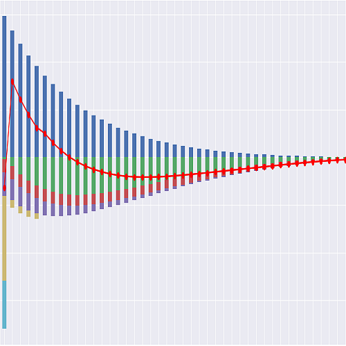
Implementation Notes#

Status: Draft, 2026-08-14. Built from products/whole_life/technical-notes.md; the product it implements is specified in product-spec.md.

This is a mechanics demonstration, not a pricing or reserving result. Very little of this product is public. The contractual skeleton is sourced — the 4.00% guarantee interest rate, endowment of the guaranteed cash value at face at age 100, the fixed 6.00% loan rate with direct recognition, paid-up additions as the default dividend option, and, for the final-expense variant, the per-$1,000 premium rates, the $36 policy fee and the 110%-of-premiums graded death benefit. Everything else is a std standardization, including all four guarantee-basis tables: the shipped mortality, net single premiums, nonforfeiture net level premiums and cash value schedules are illustrative curves calibrated to the worked example’s anchors, not the 2017 CSO / 4% tables the notes name — those are licensed and cannot be shipped here. They are not even one basis between them, because the worked example’s own anchors rule that out; the arithmetic is below. Replace them with company data before drawing any conclusion from the numbers.

Run it#

python products/whole_life/run.py
python products/whole_life/run.py 12      # the final-expense graded plan

Three lines to the same thing:

import modelx as mx
model = mx.read_model("products/whole_life/WholeLife_US_S")
model.Projection[1].result_cf()

Projection takes a point_id; Projection[1] is the worked-example anchor cell. result_cf() returns a tidy DataFrame indexed by the 0-based month index t with one column per cash flow line, the start-of-month pols_if each row is weighted by, and the net flow under both signs — net_cf (income positive, the library convention) and liability_cf (outgo positive, the notes’). result_cf_annual() sums the same frame into policy years; result_pols() and result_cv() give the decrement and value rolls.

The model and both its Spaces carry docstrings — model.doc describes the product and the projection basis, and model.Projection.doc holds the full mapping between the technical notes’ symbols and the cells names.

Monthly, and `t` is 0-based#

t counts policy months from issue, 0-based — lifelib’s own clock (basiclife/BasicTerm_S, savings/CashValue_SE) and the one every other model in this library runs on: t = 0 is the issue month, period t runs from time t to time t + 1, and for t in range(proj_len()) is the frame.

Everything contractual about this product is nevertheless annual — the guaranteed cash value schedule, the dividend declaration, the anniversary capitalization of loan interest, the premium-paying period — so the policy year is derived and used as a lookup key: duration(t) = t // 12 is the completed policy years, the contractual policy year is the 1-based label duration(t) + 1 (never indexed by), age(t) = age_at_entry() + duration(t) is the attained age entering that policy year, and age_anniv(t) the age at the anniversary ending it. is_anniv(t) — true in the last month of a policy year — is where every annual event lands.

The frame is t = proj_start() … proj_len() − 1. proj_len() = 12 × (100 − age_at_entry()) is the number of policy months projected from issue — the exclusive end of the frame, so proj_len() − 1 is the final month, the one ending at attained age 100 — and proj_start() = 12 × duration_inforce() is 0 for new business and the elapsed policy years in months for an in-force point, so the frame always opens on an anniversary. len(result_cf()) == proj_len() − proj_start(): 660 rows for the new-business male 45, 552 for the anchor at duration 9.

Two speeds, and what actually changed#

mort_rate(t) and lapse_rate(t) are the annual rates of the policy year containing month t — the vectors the notes tabulate — and mort_rate_mth(t) and lapse_rate_mth(t) are 1 − (1 − q)^(1/12), the rates the month applies. That naming is the library’s convention and tests/test_model_conventions.py asserts it. Because twelve monthly rates compound back to the annual one and every annual event stays on the anniversary, pols_if(12k) is exactly what the annual-step model carried at t = k, to floating point, and so is every anniversary-dated value: the guaranteed cash value, the dividend and all three of its margins, the paid-up additions purchased and in force, the anniversary surrender and death benefit amounts. All fifteen steps of the notes’ worked example are anniversary quantities, which is why the walk-through survived the change of grid unaltered — only the indices it is read at moved, CV_8 → CV_107 and CV_9 → CV_119.

What the finer grid buys is everything that is not contractually annual:

	Annual grid	Monthly grid
Death claims	at the anniversary, on the anniversary in force	at the end of the month of death
Surrenders	at the anniversary, valued at the anniversary CV	at the end of the month, valued at an interpolated CV
Maintenance expense	once a year, `1.02^t`	a twelfth a month, `1.02^(t/12)`
Premium	the annual premium, once a year	the modal instalment, when it is contractually due
Loan advances	one net advance a year	spread as the cash value moves; interest still capitalizes once, at the anniversary

The last of those is the one the notes themselves asked for: the annual-mode standardization of product-spec Table 2 note (f) existed only because the grid could not express the sourced modal factors, and it is now retired. premium_pp_ann(t) is the notes’ G, the annual premium; premium_pp(t) is the gross instalment billed and premium_net_pp(t) the one actually collected once any dividend offset is applied, and modal_factor_par_* / modal_factor_fe_* carry the two sourced scales ([S1] 0.515 / 0.26265 / 0.085833 and [S7] 0.52 / 0.275 / 0.089), one Reference each. The dividend offset under REDUCE_PREM is applied to the annual premium and the instalments split what is left std, so changing the mode moves the timing of the collection and not the amount the offset absorbs.

The two interpolations#

cv_pp(t) and nsp_mth(t) are straight-lined between anniversary values, (k + 1)/12 of the way with k = duration_mth(t) % 12, both std and both exact at the anniversary. cv_pp_anniv(y) is the schedule as printed, and is what the tests pin. Nothing else is interpolated: pua_face is a step function that moves only when a purchase is made, and the dividend is annual by contract.

Closing balances and opening state#

The value state variables are closing balances. cv_pp(t), pua_face(t), pua_cv(t), div_accum(t) and loan_bal(t) are all as at the end of month t. The value entering month t is the closing value of month t − 1, or, at the first projected month, the model point’s opening state — the notes’ initializations PUAF = puaf_inforce, DA = 0, L = loan_inforce. That is written inline wherever an opening balance is read,

puaf = pua_face(t - 1) if t > proj_start() else puaf_inforce()

so that no cells is ever asked for a month below the first projected one — there is no t = −1 anywhere in the model, and for an in-force point the opening balance is the model point’s input rather than a projected value. An annual quantity reads the balance entering its policy year instead, twelve months back: div_int(t) takes cv_pp(t − 12) and loan_bal(t − 12), which is the annual grid’s t − 1 under the month index.

pols_if(t) is on the same clock: the number in force at the start of month t — the notes’ l_t, l_0 = 1 at issue. See below.

Within the month the order is the notes’: premium, rider premium, premium tax and expenses at the beginning; then deaths, and — where the month is an anniversary — loan-interest capitalization and the dividend credit, then surrenders and, in the final month only, maturity at the end. So deaths carry the paid-up additions entering the month while surrenders carry the closing ones, including any dividend just credited.

Inputs are external files#

The six input CSVs live in this directory, beside run.py — not inside the model folder. WholeLife_US_S/ holds nothing but formulas:

products/whole_life/
  model_point_table.csv        <- inputs live here
  cv_table.csv
  nsp_table.csv
  np_guar_table.csv
  mort_table.csv
  premium_rates.csv
  run.py
  README.md
  WholeLife_US_S/                 <- formulas only
    __init__.py                   (model docstring)
    _system.json
    Data/__init__.py              (reads the CSVs, once per model)
    Projection/__init__.py        (the by-policy projection)

This follows lifelib’s annuallife/TradLife_A, which keeps input.xlsx beside the model and reads it at run time. It is the opposite of basiclife/BasicTerm_S, which stores its inputs inside the model through modelx’s IOSpec machinery — hence no _data/ directory and no embedded values here at all.

Read once, in `Data`#

Projection is parameterized by point_id, so every Projection[N] is a separate ItemSpace with its own cells cache. Readers placed there would re-read every file for every policy. They live instead in an unparameterized Data Space, which Projection references as data — so each file is read once per model no matter how many policies are projected, and Projection[1].data is Projection[2].data. A test counts the reads.

Data.input_dir() resolves the location from _model.path.parent when the model is read, so it works wherever the repository is checked out. Each table has a filename Reference and a reader Cells, both on Data:

Reference	Cells	File
`model_point_file`	`model_point_table()`	`model_point_table.csv`
`cv_file`	`cv_table()`	`cv_table.csv`
`nsp_file`	`nsp_table()`	`nsp_table.csv`
`np_guar_file`	`np_guar_table()`	`np_guar_table.csv`
`mort_table_file`	`mort_table()`	`mort_table.csv`
`premium_rates_file`	`premium_rates()`	`premium_rates.csv`

The trade-off: the model is not portable on its own. Copy WholeLife_US_S/ without the CSVs and it will read fine, then fail on first evaluation. What you gain is that a diff of the model shows logic changes only, and an input can be edited or swapped in place — point Data.mort_table_file at another same-schema file and the projection follows, with no formula change.

File	Contents	Provenance
`model_point_table.csv`	Fifteen points. Point 1 is the worked-example anchor cell (WL_PAR / M45 / STD_NT / $100k / $1,800 / PUA / annual mode), carried as an in-force point at duration 9 with $4,100 of paid-up additions; points 2–10 are the same policy as new business under each dividend option, each in-scope rider, the limited-pay variant and the female cell; points 11–13 are the final-expense variant; point 14 is the term blend with no rider premium funding it; point 15 is point 2 on monthly premium mode, added with the monthly grid	anchor from the worked example std; FE points from the sourced rate table [S7]; modal factors [S1] [S7]
`cv_table.csv`	Guaranteed cash value per $1,000 of face by premium period, sex, issue age and policy year, with a `provenance` column	policy years 9 and 10 of the M45 pay-to-100 cell — the model’s `cv_pp_anniv(9)` and `cv_pp_anniv(10)`, reached at `cv_pp(107)` and `cv_pp(119)` — are the worked example’s std anchors; the rest is a monotone std shape reaching exactly 1,000.00 at attained age 100. Sex-distinct throughout: the female pay-to-100 schedule is the male schedule’s funding-progress shape `f = CV^anniv / (F · NSP_{x+dur+1})` applied to the female paid-up value `F · NSP^F_{x+dur+1}` std, so it endows at face like the male one but sits below it at every earlier duration
`nsp_table.csv`	Endowment-at-100 net single premium per 1 of paid-up face by sex and age	age 55 male is the worked example’s 0.42 std; the curve is std generated and equals exactly 1.000000 at age 100. It is not the endowment NSP implied by `mort_table.csv` at 4% — see below
`np_guar_table.csv`	Nonforfeiture net level premium per $1,000 by sex and issue age, keyed by premium period	the M45 pay-to-100 cell is the worked example’s 13.00 std; the rest is `1000 · NSP_x / ä_{x:(100−x)}` on the shipped basis std, the notes’ definition. That subscript is the endowment period, not the premium period `m` — the notes annotate only the other nonforfeiture quantity, `P_adj`, with “(m = premium period)” — so `NNLP` does not vary with `m`, and the shipped rows for one (sex, issue age) are all equal. The `premium_period` key is kept so that a carrier table which does vary by `m` drops in with no formula change
`mort_table.csv`	Guaranteed mortality `q^g` by sex and age 18–100	male age 54 is the worked example’s 0.00320 std; the rest is a std illustrative Makeham curve with a 3-year female setback — not a published table, and not the 2017 CSO
`premium_rates.csv`	Final-expense annual premium per $1,000 by plan, sex, class and issue age	sourced [S7] (California edition)

What the input files key on, and why none of them moved with the index#

The 0-based time index is the model’s; the shipped CSVs were not re-keyed, because none of them is keyed by the model’s t:

File	Time-like column	Decision
`cv_table.csv`	`policy_year`, values 1 … 100 − x	Left alone. It is the contractual, 1-based policy-year label of a cash value schedule, not the frame’s index — and it stayed annual through the move to a monthly frame, because it is the contract that is annual. `cv_pp_anniv(y)` reads it directly and `cv_pp(t)` straight-lines between consecutive rows; `cv_pp_anniv(10)` is the worked example’s policy-year-10 row, 112.00 per $1,000, which `cv_pp(119)` reproduces exactly
`model_point_table.csv`	`duration_inforce`	Left alone. An elapsed count of completed policy years, which is 0-based by nature: 9 means nine years have run. `proj_start()` is `12 ×` it, so the frame opens on an anniversary
`model_point_table.csv`	`premium_mode`	Added with the monthly grid. The contractual billing mode, read by `modal_factor()` and `prem_due(t)`; point 15 is the one monthly-mode cell
`mort_table.csv`, `nsp_table.csv`	`age`	Attained age, not time; unchanged. `age(t) = x + duration(t)` and `age_anniv(t) = x + duration(t) + 1` reach them, and `nsp_mth(t)` straight-lines between two consecutive `nsp` rows
`np_guar_table.csv`, `premium_rates.csv`	`issue_age`	Issue age, not time; unchanged

No other column in any of the six files is on the frame’s time axis.

Naming#

Cells follow lifelib’s basiclife/BasicTerm_S and savings/CashValue_SE wherever those models have an analogue: pols_* for policy counts, plural nouns for cash flows, *_rate for rates, *_pp for per-policy amounts, plus model_point, age_at_entry, sum_assured, policy_term, proj_len, age, net_amt_at_risk, net_cf and result_cf, and the argument-keyed families claim_pp(t, kind), claims(t, kind) and pols_if_at(t, timing).

The technical notes use compact actuarial symbols instead; the full mapping lives in the Projection Space docstring. Seven cases needed care:

Notes	Cells	Why
`q^g`, `q^sc`, `q^e`	`mort_rate_guar` / `mort_rate_scale` / `mort_rate`	Three mortality bases off one table. `mort_rate` is the best-estimate rate that decrements the block, matching `BasicTerm_S`
`m` (premium period)	`policy_term`	It is the premium-paying period, not the coverage period — those differ on `PAY_10`
`w_t` “surrenders”	`pols_lapse`, `kind="LAPSE"`	The notes say surrenders; lifelib says lapse, and the `kind` vocabulary has to stay intact
`CSV_t`	`claim_pp(t, "LAPSE")`	The cash surrender value, not a file; reached through the shared `kind` vocabulary
`x+t` vs `x+t+1`	`age(t)` / `age_anniv(t)`	Mortality is indexed at the age entering the policy year, paid-up additions bought at its anniversary at the age one higher. Swapping them shifts every dividend purchase by a year
`q`, `w` annual	`mort_rate` / `mort_rate_mth`, `lapse_rate` / `lapse_rate_mth`	The library’s two-speed convention: the unsuffixed cells is the annual rate the notes tabulate, the `_mth` one is what the month applies. The dividend’s mortality margin uses the annual rate, and must
`G` vs the instalment	`premium_pp_ann(t)` / `premium_pp(t)` / `premium_net_pp(t)`	The annual premium the notes call `G`, the gross instalment billed in month `t`, and the one actually collected after any dividend offset
`l_t` vs `l_{t+1}`	`pols_if(t)` / `pols_if_at(t, "AFT_DECR")`	`pols_if` is the start-of-period count library-wide, and it is the weight on its own `result_cf()` row. The end-of-period count keeps a name of its own — below
`NetCF_t`	`liability_cf(t)` / `net_cf(t)`	The notes are outgo-positive and the library is income-positive, so the stream is published under both names — below

risk_class follows this product’s notes; Term_US_S calls the same concept rate_class.

The worked example sets the PUA-block dividend aside#

The notes’ worked-example table computes its last five steps from the base-block dividend alone, and says so: “For clarity the PUA-block dividend D^PUA is omitted from this table; in the model it adds (0.02 · PUACV_107) + (0.00096 · (PUAF_107 − PUACV_107)) to the amount in step 9.”

Rather than reproduce four of the fifteen steps and quietly miss the rest, the Reference pua_div_on ships False, so the base deterministic run reproduces the worked example exactly — the same device Term_US_S uses when it ships conv_rate_base = 0 because its worked example sets conversion aside.

It is a reproduction switch, not a claim about the product. Paid-up additions are dividend-eligible, that compounding is the notes’ first-ranked sensitivity, and pua_div_on = True is the product-faithful setting: on the anchor cell it raises the policy-year-10 dividend — div_credited(119), at the anniversary — from 326.25 to 361.58 and, on the new-business point, paid-up-additions face at maturity from 83,675 to 134,042. div_pua(t) implements the notes’ formula either way, and a test asserts its value against the notes’ own parenthetical — 35.331623 on the anchor cell — so neither reading can be lost.

The dividend is rounded to the cent, and that is load-bearing#

div_round_digits = 2 rounds the base dividend before it buys paid-up additions. This looks cosmetic and is not.

The notes’ worked example adds its displayed margins — 216.00 + 85.25 + 25.00 = 326.25 — and then divides 326.25 by the net single premium to get 776.79 of paid-up additions face. The exact mortality margin is 85.248, so the unrounded dividend is 326.248, and 326.248 / 0.42 = 776.7810, which displays as 776.78. One displayed cent, because the exact value sits just below the rounding boundary — and it propagates into PUAF_119 — the model’s pua_face(119), 4,876.79 — and into the death benefit.

Declared dividends are credited in whole cents, so the model rounds; that reading makes every one of the fifteen steps reproduce. Setting div_round_digits = None turns it off, and a test pins both values so the gap cannot be closed silently in either direction. Neither is “correct”: the notes’ own arithmetic is what is ambiguous.

The anchor model point is in force, not new business#

The worked example walks through policy year 10 — the months t = 108 … 119 — of a policy that already holds 9,500 of guaranteed cash value and 4,100 of paid-up additions at the anniversary it opens on. Paid-up-additions face is a projected state variable, so the only faithful way to hold it at 4,100 is to make the anchor an in-force point: duration_inforce = 9, puaf_inforce = 4100. Both columns are in the notes’ own model-point attribute table, and this is what they are for. duration_inforce is an elapsed count of policy years and so already 0-based: proj_start() is therefore 12 × 9 = 108 for point 1 and result_cf() begins at t = 108 and ends at t = 659; point 2 is the same policy issued as new business and runs the full 660 months, t = 0 … 659.

The alternative — tuning the shipped tables until a new-business projection happened to produce 4,100 at duration 9 — would have been fitting the model to the answer.

The net flow is published under both signs: `liability_cf` and `net_cf`#

The whole-life notes print

NetCF_t = −P·l − A·l + E·l + q^e_m·l·DB + w_m·l(1−q^e_m)·CSV + D^cash·l(1−q^e_m)
          + MAT·l(1−q^e_m)·1{t=T−1}

with the sign convention stated inline: outgo positive. The other eleven reference models in products/ all define net_cf the other way round, income less outgo — the sign Term_US_S sets. One name cannot carry both without result_cf()["net_cf"] becoming uncomparable and unsummable across the library.

So the model publishes the stream twice, under two names, and both are result_cf() columns:

Cells	Sign	What a positive value means	Use it for
`liability_cf(t)`	outgo positive	money leaving the insurer	reconciling against the technical notes, which print exactly this
`net_cf(t)`	income positive	money arriving at the insurer	anything that crosses models — summing, comparing, aggregating

net_cf(t) = −liability_cf(t) exactly, and a test asserts it year by year on two model points and on the result_cf() frame. This is the pattern SPIA_US_S and DIA_US_S already use for the same clash. Nothing about the whole-life notes’ own convention is denied — it is kept under a name that does not collide with the library-wide one, because a sign error in a 55-year liability projection is invisible in any summary statistic.

The four guarantee-basis tables are not one construction, and cannot be#

The notes’ first “known modeling pitfall” is a mismatch between the cash value table and the NSP/annuity functions: if they come from different bases, PUACV ≠ PUAF at age 100 and the dividend recursion leaks. The instruction is to “regenerate all guarantee-basis quantities from one 2017 CSO / 4% source.”

The shipped tables do not do that. They are pinned to their worked-example anchors one at a time: mort_table.csv to q^g_54 = 0.00320, nsp_table.csv to NSP_55 = 0.42 and NSP_100 = 1, np_guar_table.csv to NP_g = 13.00, cv_table.csv to 95.00 and 112.00 per $1,000 on its policy-year 9 and 10 rows (cv_pp_anniv(9), cv_pp_anniv(10)). This is a disclosed divergence, not an oversight, because the worked example’s own anchors are unreachable on any single basis:

On one mortality table at interest i, endowment insurance and the annuity-due satisfy A_{x:n|} = 1 − d · ä_{x:n|} with d = i / (1 + i). The notes’ definition NNLP = F · NSP_x / ä_{x:(100−x)|} therefore collapses to

NNLP / F = d · NSP_45 / (1 − NSP_45)

and the worked example’s NNLP = 13.00 per $1,000 at i = 4% forces NSP_45 = 13 / (1000 d + 13) = 0.252616. But the endowment recursion NSP_y = v · (NSP_{y+1} + q_y (1 − NSP_{y+1})) gives NSP_y ≥ v · NSP_{y+1} for every q_y ≥ 0, so

NSP_55  ≤  NSP_45 · 1.04^10  =  0.252616 × 1.480244  =  0.373933   <   0.42

whatever mortality is assumed. Read the other way, NSP_55 = 0.42 forces NSP_45 ≥ 0.42 / 1.04^10 = 0.283737 and hence NNLP ≥ 15.236 per $1,000 — 17% above the notes’ 13.00. Steps 3 and 10 of the worked-example table are mutually exclusive.

The size of the resulting gap is worth stating plainly. Recomputing the endowment NSP from the shipped mortality at 4% gives 0.330820 at age 55 against the shipped 0.420000 (+27.0%) and 0.236184 at 45 against 0.258170 (+9.3%). Reconciling the two needs a guarantee interest rate that falls from 5.99% at age 45 to 4.89% at 54, 2.08% at 80 and 0.02% at 99 — never the 4.00% int_rate_guar that div_int credits excess interest against. Inverting the shipped curve for the implied q at 4% is worse still: the male curve implies a negative mortality rate at every age from 18 to 57 and a rate above 1 from age 89 on (female: 18–62 and 90 on). test_the_guarantee_basis_is_not_one_construction pins all of this, so the mismatch cannot quietly change size or quietly close.

What the shipped tables do guarantee are the two endpoints whose failure the pitfall is actually about, and both are asserted:

nsp = 1.000000 at attained age 100, so pua_cv(T − 1) == pua_face(T − 1) exactly, and
cv_per_1000 = 1000.00 on the last policy year of the schedule, so cv_pp(T − 1) == sum_assured(), where T = proj_len() and T − 1 is the last projected period.

Neither block leaks at maturity. What is missing is the means — one basis — not the endpoints.

Swapping in the real 2017 CSO / 4% tables means replacing all four files together; replacing mort_table.csv alone is precisely the pitfall the notes warn about, and the Data docstring says so. It also means the worked example will stop reproducing, which is the honest price of the notes’ own arithmetic rather than something to tune away.

The term-blend rider needed two decisions the notes do not make#

The notes originally gave the blend as: OYT face = max(TF − F − PUAF_t, 0), the dividend first pays q^sc · OYT_t · v_g, remainder buys paid-up additions.

It is circular. PUAF_t is bought with the dividend that is left after the term cost, which is computed from PUAF_t. The model sizes the layer on the block entering the policy year instead — pua_face(anniv − 12), or puaf_inforce() where that falls before the frame — and says so in the oyt_face docstring. The notes were rewritten to match, and now read max(TF − F − PUAF_{prev anniv}, 0) with the cost at q^{sc}_{x+dur+1} · OYT · v_g.

It has no shortfall rule. Nothing in the notes says what happens when the dividend cannot pay for the whole gap. Left uncapped, the model would report a term face it never charges for and inflate the death benefit by the difference. So the layer is capped at D_t (1 + i_g) / q^sc_{x+t+1} — as much term as the dividend actually buys — and claim_pp(t, "DEATH") is written as F + PUAF_{t−1} + OYT_t, which equals the notes’ “target face plus excess paid-up additions” whenever the gap is funded and stays correct when it is not.

Whether the cap binds is a property of the funding, not of the design, so the model carries both cases:

	Model point 8 — 2× target, $5,000 rider premium	Model point 14 — 2× target, no rider premium
cap binds in	policy year 1 only, where `div_first_year = 2` means no dividend is payable at all	policy years 1–3, while the dividend is still small, and every year from the thirtieth on as `q^sc` outruns it — 29 of 55 years
crossover	policy year 8: the rider money closes the gap and the blend becomes pure paid-up additions	never; `PUAF` reaches only 6,513 by maturity against a 100,000 gap

Point 8 is how blends are actually funded and exercises the uncapped branch; point 14 exists so the shortfall branch is exercised too, and so the claim that the block never crosses over without rider money is a test rather than an assertion.

The last REDUCE_PREM dividend has no premium left to offset#

Under REDUCE_PREM the notes route the dividend to the next policy year’s premium: G^net = max(G − D_{prev anniv}, 0), excess to paid-up additions. At the final anniversary, t = T − 1, there is no policy year after it. The notes never say what becomes of that last dividend, and reading them literally drops it: the dividend is credited, offsets nothing, buys nothing, is not paid in cash and never reaches the maturity benefit. On model point 5 that lost the final anniversary’s dividend of 2,030.14 — more than a full year’s gross premium — while the other three options all delivered theirs.

The model treats the whole of D_{T−1} as REDUCE_PREM excess and buys paid-up additions with it at NSP_100 = 1 std, which is the rule the option already applies in every year whose premium the dividend has outgrown, and which is exact at attained age 100 where a dollar of paid-up face costs a dollar. test_every_credited_dividend_is_delivered asserts the closing identity — total credited equals total delivered — for all four dividend options, so no option can silently leak a dividend again.

`pols_if` is the start-of-month count#

Every other state variable in these notes is an end-of-period value, but the in-force probability is read at the start of the period, because that is what the period’s cash flows are earned by: the notes write every term of NetCF_t over the same count that pays the premium. Reporting the end-of-period count in a pols_if column would put a policy count on a row whose cash flows belong to a different count, and the printed table would stop reconciling: 1,800 of premium beside 0.98 policies.

pols_if(t) is therefore the number in force at the start of period t — the notes’ l_t, l_0 = 1 at issue — which is both the weight on that same result_cf() row and what pols_if means in every other model in this library but SPIA_US_S (Term_US_S.pols_if(0) is pols_if_init(); lifelib’s CashValue_SE.pols_if(t) is pols_if_at(t, "BEF_MAT")). premiums(t) / premium_net_pp(t) == pols_if(t) is an identity wherever an instalment falls, and a test asserts it; pols_if(proj_start()) == pols_if_init() on every model point, in force or new business. SPIA_US_S is the library’s one documented exception: its pols_if(t) is the notes’ end-of-month obligation indicator max(C(t), l_alive(t+1)), a closing measure, so pols_if(0) != pols_if_init() there — see that product’s own model.md.

The end-of-period count is not lost. It is pols_if_at(t, "AFT_DECR"), the notes’ l_{t+1} and the fourth timing string: after deaths, surrenders and — in the final period — maturities, which is where the notes’ processing order ends. CashValue_SE has no name for that point, hence a new string rather than a reused one; it is documented in the pols_if_at docstring and pols_if_at(t, "AFT_DECR") == pols_if(t + 1) by construction.

`pols_maturity` and the terminal year#

pols_if(t) is zero from t = proj_len() onward, because everything still in force in the final projected period T − 1 matures at attained age 100 and the contract terminates. That is not a decrement — the modelled contract simply ends — but the roll-forward does not close without naming it, so pols_maturity(t) carries it, zero in every period but the last:

pols_if(t) − pols_if(t+1) = pols_death(t) + pols_lapse(t) + pols_maturity(t)

The notes’ lapse schedule cooperates: it is “0 through the final policy year”, so the survivors of the final month mature rather than surrender.

check_pols_roll_fwd() takes no argument and returns a bool over every projected period — the shape every check_* in this library has, so one test can call the same check across all twelve models — and check_pols_roll_fwd_resid(t) returns the signed residual of a single month for when it fails. check_pua_roll_fwd() / check_pua_roll_fwd_resid(t) are the same pair for the paid-up-additions block, which is this product’s analogue of CashValue_SE.check_av_roll_fwd().

Standardizations used#

Everything in this list is std: the 6.00% dividend interest rate snapshot and the whole three-factor dividend parametrization; the 0.70 experience factor, which produces both the scale mortality and the best-estimate mortality (the notes’ “consistency trap”); the $25 expense margin; the dividend floor at zero and the no-dividend-in-year-1 convention; rounding the dividend to the cent; the par lapse schedule (5% grading to 2% by year 10, level after, zero in the maturity year) and the final-expense schedule (12%, 10%, grading to 6% by year 5); acquisition expense 90% of first-year premium plus $250; maintenance $60 a year accruing at a twelfth a month and inflating at 1.02^(t/12); premium tax 2%, which the notes’ processing order collects but their one-line NetCF formula omits — the model follows the processing order; the 10% load on paid-up-additions rider payments; the 2× term-blend target and both blend decisions above; routing the final period’s REDUCE_PREM dividend to paid-up additions, since there is no premium after it to offset; the 3% accidental share of final-expense deaths; truncation of the projection at attained age 100; holding the loan at loan_utilization × CV_t; the funding-progress construction that makes the pay-to-100 cash value schedule sex-distinct; the constant-force conversion of every annual rate to its monthly counterpart; the straight-line interpolation of the cash value and the net single premium between anniversaries; applying the REDUCE_PREM offset to the annual premium and letting the instalments split what is left; and every value in cv_table.csv, nsp_table.csv, np_guar_table.csv and mort_table.csv — which, as set out above, are four separate constructions rather than one.

Switched off by default, all implemented and all one Reference away: pua_div_on (see above), dyn_lapse_on with competitor_rate (the interest-sensitive lapse multiplier), and prem_offset_on with prem_offset_share (the premium-offset behavioural overlay, applied proportionally rather than by splitting the cohort — a std simplification of the notes’ “a fraction 0.50 of policyholders switch”).

Not implemented, and named as such in the model docstring: reduced paid-up and extended term nonforfeiture, the automatic premium loan, partial surrender of paid-up additions, terminal dividends and dividends credited at death, variable and adjustable loan rates, the age 100–121 tail, state variations, and any §7702 / §7702A policing — mec_flag() flags a model point that would need the test rather than performing it, exactly as the notes prescribe.

Tests#

tests/test_whole_life_us.py asserts all fifteen steps of the worked example to the cent, the PUA-block dividend against the notes’ parenthetical, the in-force and paid-up-additions roll-forwards, the four cash-value/NSP endpoint invariants, one test per “known modeling pitfall” the notes list, the dividend-rounding divergence in both directions, both signs of the net flow and that they are exact negatives, the start-of-month meaning of pols_if and its reconciliation with its own row, each dividend option, each rider, the final-expense graded benefit and its premium formula against the sourced rates, the annual-equivalence invariant (pols_if(12k) against the annual recursion at every anniversary of the frame), that the two interpolations are exact at the anniversary and that no annual event is credited off one, the modal-premium machinery against model point 15, result_cf() shape, and that all fifteen model points project. Four of them pin the divergences and the decisions written up above so they cannot quietly change:

Test	Pins
`test_the_guarantee_basis_is_not_one_construction`	the impossibility arithmetic, and the implied guarantee interest rate by age — the size of the mismatch between `nsp_table.csv` and `mort_table.csv`
`test_np_guar_is_the_notes_endowment_period_net_level_premium`	`NP_g` recomputed from `mort_table.csv` and `nsp_table.csv` as `1000 · NSP_x / ä_{x:(100−x)}`, and that it does not vary with the premium period
`test_cv_schedule_is_sex_distinct`	the female schedule below the male at every duration, equal at maturity, on every premium period
`test_every_credited_dividend_is_delivered`	total dividend credited = total delivered, under each of the four dividend options, including the final year

python -m pytest tests/test_whole_life_us.py -q

Verifying this copy#

tests/test_whole_life_us.py asserts this model against the worked example in technical-notes.md, and it ships inside this library — so it runs against the copy you are holding, including any changes you have made to it:

python -m pytest tests/test_whole_life_us.py -q

The whole suite, all twelve models and the shared conventions, is python -m pytest tests -q. If you change an assumption and a test goes red, the worked example in the notes and the model have parted company — which is the question this library exists to let you ask.