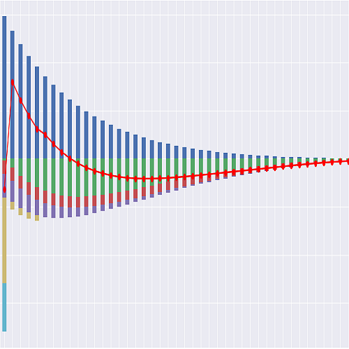
The Projection Space

The by-policy projection of the WholeLife_US_S model.

The Space is parameterized by point_id, so Projection[1] is an ItemSpace projecting model point 1:

>>> Projection[1].result_cf()          # the worked example's anchor cell
>>> Projection.point_id = 2            # or switch the default

Input data

Inputs are external files: plain CSVs living in the model folder’s parent directory, products/whole_life/, read at run time rather than stored inside the model. The model folder therefore holds nothing but formulas — no _data/, no IOSpec, no embedded values — so a diff of the model shows logic changes only, and an input can be edited or swapped without rewriting the model. This follows annuallife.TradLife_A; contrast basiclife.BasicTerm_S, which keeps its inputs inside the model through modelx’s IOSpec machinery.

The consequence worth knowing: the model is not portable on its own. Copying the WholeLife_US_S folder without its parent’s CSVs produces a model that reads and then fails on first evaluation.

Each table has a filename Reference and a reader Cells, both on the Data Space, reached here through the data Reference:

Reference	Cells	File
model_point_file	data.model_point_table()	model_point_table.csv
cv_file	data.cv_table()	cv_table.csv
nsp_file	data.nsp_table()	nsp_table.csv
np_guar_file	data.np_guar_table()	np_guar_table.csv
mort_table_file	data.mort_table()	mort_table.csv
premium_rates_file	data.premium_rates()	premium_rates.csv

The time index

t counts policy months from issue, 0-based — lifelib’s own clock (basiclife.BasicTerm_S, savings.CashValue_SE) and the one every other model in this library runs on. t = 0 is the issue month, period t runs from time t to time t + 1, and proj_len() = 12 * (100 - x) is the number of policy months projected, the exclusive end of the frame: the projection runs t = proj_start() .. proj_len() - 1. proj_start() is 0 for new business and 12 * duration_inforce() — the policy years already elapsed, in months — for an in-force model point, so pols_if(proj_start()) is pols_if_init().

Everything contractual about this product is on an annual cycle: the guaranteed cash value schedule, the dividend declaration, the anniversary capitalization of loan interest, the premium-paying period. The policy year is therefore derived and used as a lookup key throughout — duration(t) = duration_mth(t) // 12 is the completed policy years at the start of month t, policy_year(t) = duration(t) + 1 is the contractual 1-based label (the policy_year key of cv_table.csv), age(t) = age_at_entry() + duration(t) is the attained age entering that policy year and age_anniv(t) the age at the anniversary that ends it. is_anniv(t) is true in the last month of a policy year, which is where every annual event lands.

The value state variables are closing balances at the end of month t: cv_pp(t), pua_face(t), pua_cv(t), div_accum(t) and loan_bal(t). The value entering month t is the closing balance of month t - 1, or, at the first projected month, the model point’s opening state (puaf_inforce(), loan_inforce(), zero accumulation, and a guaranteed cash value of zero at issue) — written inline as pua_face(t - 1) if t > proj_start() else puaf_inforce() wherever an opening balance is read, so that nothing is ever indexed below the first projected month. Annual quantities read the balance entering the policy year instead, twelve months back.

What the monthly grid changes, and what it does not

Decrements run in two speeds, the library’s convention: mort_rate(t) and lapse_rate(t) are the annual rates of the policy year containing month t — the vectors the technical notes tabulate — and mort_rate_mth(t) and lapse_rate_mth(t) are the monthly rates actually applied, 1 - (1 - q)^(1/12). Twelve of those compound back to exactly the annual rate, so the in-force at every policy anniversary is what an annual-step model would carry, to floating-point.

The annual events stay annual and land on is_anniv(t): the dividend is declared and credited once a year, at the anniversary; loan interest capitalizes there; paid-up additions are bought with the dividend there. What the finer grid buys is everything that is not contractually annual — death claims settle at the end of the month of death rather than the end of the policy year, maintenance expense accrues monthly, the guaranteed cash value and the paid-up-additions cash value interpolate between anniversaries so a mid-year surrender is valued where it happens, and a modal premium is collected when it is contractually due. That last one is why the technical notes’ “premium mode modeled: annual” [std] is retired: the modal factors are sourced ([S1] for the participating design, [S7] for final expense) and the monthly grid is what makes them expressible. result_cf_annual() sums the frame into policy years so a monthly run can be laid beside an annual one.

Two interpolations are standardizations introduced here, both [std] and both exact at the anniversary so that no anniversary quantity moves:

cv_pp(t)

Straight-line between the schedule’s anniversary values, (k + 1) / 12 of the way from the value at the anniversary opening the policy year to the value at the one closing it, k = duration_mth(t) % 12. Contractual cash value tables are printed at anniversaries only [S1] [S3]; pro-rating for elapsed time is the ordinary policy-form convention and the Standard Nonforfeiture Law requires some adjustment for it.

nsp_mth(t)

The same straight line applied to the net single premium between NSP_{x+dur} and NSP_{x+dur+1}, so the paid-up-additions block is valued on the same clock as the base cash value.

Naming

Cells names follow lifelib’s basiclife.BasicTerm_S and savings.CashValue_SE wherever those models have an analogue — pols_* for policy counts, plural nouns for cash flows, *_rate for rates, *_pp for per-policy amounts, claim_pp(t, kind) and pols_if_at(t, timing) for the argument-keyed families. The technical notes use compact actuarial symbols instead. The mapping is:

Notes symbol	Cells	Meaning
x	age_at_entry	Issue age (ANB)
x + dur	age(t)	Attained age entering the policy year of month t
x + dur + 1	age_anniv(t)	Attained age at the anniversary ending it
T = 12(100 - x)	proj_len	Policy months projected
t0	duration_inforce	Policy years already elapsed
12 t0	proj_start	First projected month
(t // 12)	duration(t)	Completed policy years
	duration_mth(t)	Completed policy months
dur(t)	policy_year(t)	Policy year, duration(t) + 1
(anniversary)	is_anniv(t)	Last month of a policy year
m	policy_term	Premium-paying period, years
F	sum_assured	Base face amount
G	premium_pp_ann(t)	Gross annual premium
(modal)	premium_pp(t)	Premium due in month t
(modal factor)	modal_factor	Fraction of G per instalment
(modal cycle)	prem_cycle	Months between instalments
(due month)	prem_due(t)	Whether an instalment is due
G^net_t	premium_net_pp_ann(t)	Annual premium after offset
(modal)	premium_net_pp(t)	The instalment actually collected
A_t	rider_premium_pp_ann(t)	PUA rider premium, annual
(modal)	rider_premium_pp(t)	The instalment due in month t
i_g	int_rate_guar	Guarantee interest, 4.00%
i_d	int_rate_div	Dividend interest rate, 6.00%
i_L	int_rate_loan	Policy loan rate, 6.00%
q^g_{x+t}	mort_rate_guar(t)	Guarantee mortality, annual
q^g_y	mort_rate_guar_at(y)	The same, keyed by age
q^sc_{x+t}	mort_rate_scale(t)	Dividend-scale mortality
q^e_{x+t}	mort_rate(t)	Best-estimate mortality, annual
(q^e monthly)	mort_rate_mth(t)	The monthly rate applied
w_t	lapse_rate(t)	Surrender rate, annual
(w monthly)	lapse_rate_mth(t)	The monthly rate applied
w^dyn multiplier	dyn_lapse_factor(t)	Interest-sensitive overlay
l_t	pols_if(t)	In force at BOM t (weight)
l_{t+1}	pols_if_at(t, “AFT_DECR”)	In force at EOM t
l_t(1-q^e)	pols_if_at(t, timing)	In force inside month t
(none)	pols_death(t)	Deaths in month t
(none)	pols_lapse(t)	Surrenders at EOM t
(none)	pols_maturity(t)	Maturities at T - 1
CV_t	cv_pp(t)	Guaranteed cash value, EOM t
CV at anniversary	cv_pp_anniv(y)	The schedule’s own values
F - CV_t	net_amt_at_risk(t)	Guarantee net amount at risk
NSP_y	nsp(y)	Net single premium, endow 100
(NSP monthly)	nsp_mth(t)	NSP interpolated to EOM t
NP_g	np_guar()	Nonforfeiture net level premium
D^int_t	div_int(t)	Interest margin
D^mort_t	div_mort(t)	Mortality margin
D^exp_t (e^m_t)	div_exp(t)	Expense margin
D_t	div_base(t)	Base-block dividend, floored
D^PUA_t	div_pua(t)	PUA-block dividend
D_t + D^PUA_t	div_credited(t)	Dividend credited at EOM t
D_{t-1}	div_prev_anniv(t)	Dividend at the anniversary opening the policy year of t
D^cash_t	div_cash(t)	Cash dividend per policy
(none)	div_to_pua(t)	Dividend applied to PUAs
dPUAF_t	pua_face_purch(t)	PUA face bought by dividend
dPUAF^rider_t	pua_face_rider(t)	PUA face bought by the rider
(none)	pua_face_offset(t)	PUA face from the RPD excess
PUAF_t	pua_face(t)	PUA face in force at EOM t
PUACV_t	pua_cv(t)	PUA cash value at EOM t
DA_t	div_accum(t)	Dividend accumulation balance
L_t	loan_bal(t)	Loan balance at EOM t
(none)	loan_int(t)	Loan interest capitalized
(none)	loan_draw(t)	Net new borrowing per policy
TF	term_blend_target	Term-blend target face
OYT_t	oyt_face(t)	One-year-term face in the blend
(none)	oyt_cost(t)	Dividend absorbed by the OYT
DB_t	claim_pp(t, “DEATH”)	Death benefit per policy
CSV_t	claim_pp(t, “LAPSE”)	Surrender value per policy
MAT	claim_pp(t, “MATURITY”)	Maturity benefit per policy
(none)	prem_cum(t)	Cumulative premiums paid
E_t	expenses(t)	Acquisition + maintenance
(none)	premium_taxes(t)	Premium tax outgo
(none)	premiums(t)	Premium income
(none)	rider_premiums(t)	PUA rider premium income
(none)	claims(t, kind)	Benefit outgo
(none)	div_cash_paid(t)	Cash dividend outgo
(none)	loan_draws(t)	Net loan advances
NetCF_t	liability_cf(t)	Net liability CF, outgo +
(none)	net_cf(t)	The same, income positive
(none)	result_cf_annual()	result_cf() summed into years

Seven names needed care.

mort_rate is the best-estimate rate — the one that actually decrements the block — while the guarantee and dividend-scale rates are mort_rate_guar and mort_rate_scale. All three come off the same shipped table through the References ae_best_est and ae_scale. The notes call this out as a consistency trap: the same table feeds claim outgo and the dividend’s mortality margin with opposite signs, so raising best-estimate mortality raises claims and, if the scale factor moves with it, cuts the dividend.

policy_term is the premium-paying period m in years, not the coverage period. Coverage runs to proj_len() in every variant; on the base pay-to-100 design the two coincide, on PAY_10 they do not. It stays in years because the contract states it in years; premium_pp compares it against duration(t).

pols_lapse counts surrenders. The notes say “surrenders”, BasicTerm_S says pols_lapse, and CashValue_SE’s kind string is "LAPSE"; the model keeps the lifelib name so the kind vocabulary stays intact.

The notes’ CSV_t is the cash surrender value, not a file. It is reached as claim_pp(t, "LAPSE") so that all three benefit amounts share one cells and one kind vocabulary with CashValue_SE.

age(t) and age_anniv(t) are both needed: the notes index mortality at the attained age entering the policy year but price paid-up additions bought at the end of it one year later. Getting them the wrong way round shifts every dividend purchase by a year.

pols_if(t) is the start-of-month count — the notes’ l_t, not their l_{t+1}. That is the library-wide convention (Term_US_S.pols_if(0) is pols_if_init(), CashValue_SE.pols_if(t) is pols_if_at(t, "BEF_MAT")), and it is the number every cash flow on the same result_cf() row is weighted by. The notes’ end-of-period state variable is not lost — it is pols_if_at(t, "AFT_DECR"), and pols_if_at(t, "AFT_DECR") == pols_if(t + 1) by construction.

liability_cf(t) and net_cf(t) are the same stream with opposite signs — see the sign-convention rubric below.

Timing and kind arguments

pols_if_at(t, timing) takes "BEF_DECR" (start of month t, before any decrement — the same number as pols_if(t)), "BEF_SURR" (after deaths, before surrenders), "BEF_MAT" (after surrenders, before maturity) and "AFT_DECR" (after every decrement, the notes’ l_{t+1}) — the notes’ end-of-period processing order, deaths then dividend then surrenders then maturity, now applied every month. "BEF_DECR" and "BEF_MAT" are CashValue_SE’s names; "BEF_SURR" is added because this product settles deaths and surrenders in one end-of-period step, and "AFT_DECR" because CashValue_SE has no string for the point past the last decrement, which is where the notes’ state variable lives. claim_pp(t, kind) and claims(t, kind) take "DEATH", "LAPSE" and "MATURITY". Both raise ValueError("invalid timing") / ValueError("invalid kind") on anything else.

The dividend is rounded to the cent

div_round_digits = 2 rounds the credited base dividend before it buys paid-up additions. This is [std], and it is not cosmetic: the notes’ worked example adds the displayed margins (216.00 + 85.25 + 25.00 = 326.25) and then divides 326.25 by the net single premium. Carrying the unrounded 326.248 through instead moves the purchased paid-up-additions face from 776.79 to 776.78 — a full displayed cent, because the exact value sits just under the rounding boundary. Declared dividends are credited in whole cents, so the model rounds; setting div_round_digits = None turns it off and a test pins the size of the gap in both directions.

The worked example sets the PUA-block dividend aside

The notes’ worked-example table computes steps 11-15 from the base-block dividend alone, saying so explicitly: “For clarity the PUA-block dividend D^PUA is omitted from this table; in the model it adds … to the amount in step 9.” The Reference pua_div_on ships False so the base deterministic run reproduces the worked example exactly, the same way Term_US_S ships conv_rate_base = 0. It is a reproduction switch, not a claim that paid-up additions are excluded from the dividend — they are dividend-eligible, and pua_div_on = True is the product-faithful setting. div_pua(t) implements the notes’ formula either way, and a test asserts its value on the anchor cell against the notes’ own parenthetical.

The four guarantee-basis tables are not one construction

The notes’ first “known modeling pitfall” is a mismatch between the cash value table and the NSP/annuity functions, and prescribes regenerating every guarantee-basis quantity from one 2017 CSO / 4% source. The shipped tables do not satisfy that, and no set of tables carrying the worked example’s anchors could. On any single mortality basis at interest i, endowment insurance and the annuity-due satisfy A_{x:n} = 1 - d ae_{x:n} with d = i/(1+i), so the notes’ own definition collapses to NNLP = 1000 d NSP_45 / (1 - NSP_45); the worked example’s NNLP = 13.00 then forces NSP_45 = 0.252616. But NSP_y = v(NSP_{y+1} + q_y (1 - NSP_{y+1})) >= v NSP_{y+1} for any q_y >= 0, so NSP_55 <= NSP_45 (1.04)^10 = 0.373933 — below the worked example’s NSP_55 = 0.42. Read the other way: NSP_55 = 0.42 forces NSP_45 >= 0.283737 and hence NNLP >= 15.236 per $1,000, 17% above the notes’ 13.00. The worked example’s steps 3 and 10 are mutually unreachable, whatever mortality table is used.

What the shipped tables do instead [std]: mort_table.csv is an illustrative Makeham curve pinned to q^g_54 = 0.00320; nsp_table.csv is a separate parametric curve pinned to NSP_55 = 0.42 and NSP_100 = 1; np_guar_table.csv holds 1000 NSP_x / ae_{x:(100-x)} with the annuity taken on the mortality table’s own survivorship, which is what makes NP_g = 13.00; and cv_table.csv is a monotone shape solved through its policy-year 9 and 10 rows — the worked example’s 95.00 and 112.00 per $1,000, which are cv_pp_anniv(9) and cv_pp_anniv(10) — to 1000.00 at attained age 100. Reconciling the NSP curve with the mortality table needs a guarantee interest rate that falls from 5.99% at age 45 to 0.02% at age 99, and inverting the curve for the implied q at 4% gives a negative rate at every age up to 57 and a rate above 1 from age 89 on.

The two consequences the pitfall names are nevertheless absent, and are asserted by tests: NSP_100 = 1 exactly, so pua_cv(T - 1) == pua_face(T - 1), and the schedule reaches exactly face in the final policy month, so cv_pp(T - 1) == sum_assured(), where T = proj_len() and T - 1 is the last projected month. Neither block leaks at maturity. What is missing is the means — one basis — not the endpoints. Swap in a licensed 2017 CSO / 4% set and all four files must be replaced together; the worked example will then no longer reproduce, which is the honest price of the notes’ own arithmetic.

Sign convention — two names, one stream

The whole-life notes print NetCF_t with outgo positive, which is the opposite of the sign the other eleven reference models in products/ carry. Rather than pick one and lose the other, the model publishes both and names them apart:

liability_cf(t)

The notes’ NetCF_t, verbatim: outgo positive. Premium and rider income enter with a minus sign; expenses, premium tax, claims, cash dividends and net loan advances enter with a plus. A positive liability_cf is money leaving the insurer. This is the number to compare against the notes.

net_cf(t)

-liability_cf(t): income positive, the sign convention every model in products/ carries, so that result_cf()["net_cf"] can be summed or compared across products. A positive net_cf is money arriving at the insurer.

Both are columns of result_cf(). The pattern is SPIA_US_S and DIA_US_S’s, which face the same clash. Nothing about the whole-life notes’ own convention is being denied — it is being kept under a name that does not collide with the library-wide one, because a sign error in a 55-year liability projection is invisible in a summary statistic.

Cells Descriptions

model_point()

The selected model point as a Series.

product()

The product code: WL_PAR, WL_FE_LEVEL or WL_FE_GRADED.

is_par()

True for the participating design, which is the only one that pays dividends.

premium_period()

The premium period code: TO_100, PAY_10, PAY_20 or TO_65.

age_at_entry()

The issue age (ANB) of the selected model point.

sex()

The sex of the selected model point; rates are sex-distinct throughout.

risk_class()

The underwriting class of the selected model point (PREF_NT / STD_NT / TOB).

sum_assured()

The base face amount F of the selected model point.

dividend_option()

The elected dividend option: PUA, CASH, ACCUM, REDUCE_PREM, or NONE for non-par.

premium_mode()

The premium mode of the selected model point: A, SA, Q or M.

The technical notes’ “premium mode modeled: annual” was a consequence of the annual grid, not of the contract: every design in the spec is sold on all four modes [S1] [S7]. On the monthly grid the mode is a model point attribute, and the shipped table exercises both ends of it.

pols_if_init()

Initial number of policies in force, l at proj_start().

duration_inforce()

t0: policy years already elapsed at the valuation date; 0 for new business.

The contract states elapsed time in policy years and so does the model point table; proj_start() turns it into the month the frame opens at.

puaf_inforce()

PUAF at t0: paid-up additions face already in force at the valuation date.

loan_inforce()

L at t0: policy loan balance already outstanding at the valuation date.

loan_utilization()

Fraction of the guaranteed cash value held as a policy loan [std].

0 in the base run; the notes’ variant is 0.20, maintained by borrowing and repaying as the cash value moves.

term_blend_target()

TF: the term-blend rider’s target face amount; 0 switches the rider off.

is_blended()

True when the term-blend rider is active on this model point [std].

The blend needs the dividend to pay the one-year-term cost, so it is modelled only under the PUA dividend option and only on the participating design.

proj_len()

T = 12 (maturity_age - x): the number of policy months projected from issue.

The exclusive end of the frame, counted from t = 0: the projection runs t = proj_start() .. proj_len() - 1, so proj_len() - 1 is the last projected month, the one ending at attained age 100.

The contract itself matures at 121, but the guaranteed cash value equals face at 100 and the paid-up-additions cash value equals paid-up-additions face there, so from 100 the policy is economically an endowment at face. Truncating at 100 is a [std] simplification that moves the age 100-121 payments from death to maturity without changing their amount per survivor.

proj_start()

The first projected month, 12 * duration_inforce().

New business starts at t = 0; an in-force model point starts at the month its elapsed policy years end, so duration_inforce = 9 opens the frame at t = 108, the first month of the tenth policy year. Elapsed time is recorded in whole policy years, so the frame always opens on an anniversary.

policy_term()

m: the premium-paying period in years, from the premium period code.

This is not the coverage period, which is proj_len() in every variant. It stays in years because the contract states it in years; premium_pp_ann() compares it against duration(t).

duration_mth(t)

Completed policy months at the start of month t.

t itself: every model point is projected on the policy’s own clock, and an in-force point opens the frame at proj_start() rather than re-basing t. The cells exists so the monthly vocabulary reads the same here as in the UL family and savings.CashValue_SE.

duration(t)

Completed policy years at the start of month t, duration_mth(t) // 12.

0 throughout the first policy year. Every contractual schedule in this product is annual, so this is what the attained age, the cash value schedule, the premium period and the decrement vectors are all read at.

policy_year(t)

The contractual policy year containing month t, duration(t) + 1.

A 1-based label derived from t, never indexed by: it is the policy_year key of cv_table.csv.

is_anniv(t)

True in the last month of a policy year, where every annual event lands.

The dividend is declared and credited here, loan interest capitalizes here, and paid-up additions are bought here. duration_mth(t) % 12 == 11.

anniv_mth(t)

The month index of the anniversary that ends the policy year containing t.

12 * duration(t) + 11, which is t itself when is_anniv() is true. Used by the term-blend layer, which is bought at that anniversary and is in force for the whole of the policy year it closes.

age(t)

The attained age x + duration(t) entering the policy year containing month t.

Mortality in that policy year is indexed here; paid-up additions bought at the anniversary that ends it are priced at age_anniv(t).

age_anniv(t)

The attained age at the anniversary that ends the policy year containing month t.

mec_flag()

True where the model point would need a Sect. 7702A test this model does not run.

The notes are explicit that the reference model does not police Sect. 7702 or Sect. 7702A limits and should flag model points that would fail rather than silently projecting them [std]. Limited-pay designs sit near the 7-pay limit and paid-up-additions rider payments consume 7-pay room, so both raise the flag.

premium_rate()

Final-expense annual premium per $1,000 of face, from premium_rates.csv [S7].

modal_factor()

The fraction of the annual premium collected per instalment [S1] [S7].

The participating design takes the [S1] scale — semi-annual 0.515, quarterly 0.26265, monthly 0.085833 — and the final-expense variant the [S7] scale printed on its own rate card — 0.52, 0.275, 0.089. Both are sourced, and both carry the modal loading inside the factor, so twelve monthly instalments come to 1.03 of the annual premium on the participating design and 1.068 on final expense. Each factor is its own Reference, so a carrier’s own scale drops in without a formula change.

prem_cycle()

Months between premium instalments: A 12, SA 6, Q 3, M 1.

Arithmetic of the mode rather than an assumption, so it is written here rather than held in a Reference.

prem_due(t)

Whether a modal premium instalment falls due at the beginning of month t.

Instalments start on the policy anniversary and repeat on the mode’s own cycle: annual in the first month of each policy year, semi-annual every sixth month, quarterly every third, monthly every month.

premium_pp_ann(t)

G: the gross annual premium per policy for the policy year containing month t.

Level and guaranteed through the policy_term() premium-paying years duration(t) = 0 .. policy_term() - 1, zero after. The participating design takes G from the model point ([std illustrative] — carrier rate books are not public); the final-expense variant computes it from the sourced rate table as (F / 1000) * rate(x, sex, class) + 36 [S7].

This is the notes’ G and the base for the acquisition expense, the premium offset and the paid-up-additions purchases, none of which should move with the premium mode; premium_pp() is what is actually collected in month t.

premium_net_pp_ann(t)

G^net_t: the annual premium actually charged for the policy year of month t.

Under REDUCE_PREM the dividend credited at the anniversary opening that policy year offsets the premium, max(G - D, 0), and any excess buys paid-up additions through pua_face_offset(). The dynamic premium-offset overlay ([std], off by default) applies a prem_offset_share fraction of the same offset once the dividend has grown to cover the premium.

premium_pp(t)

The gross premium instalment per policy due at the beginning of month t.

modal_factor() * G in an instalment month, zero otherwise: what the policy is billed before any dividend offset. premium_net_pp() is what is actually collected, and the two differ only under REDUCE_PREM and the premium-offset overlay.

premium_net_pp(t)

The premium per policy actually collected at the beginning of month t.

modal_factor() * G^net in an instalment month, zero otherwise. The dividend offset is applied to the annual premium and the instalments then split what is left [std], so a mode change moves the timing of the collection and not the amount the offset absorbs. This is what premiums() is weighted from.

rider_premium_pp_ann(t)

A_t: the annual paid-up-additions rider premium for the policy year of month t.

Level while base premiums are payable [std]; the notes set it within limits fixed at issue and do not schedule it.

rider_premium_pp(t)

The paid-up-additions rider instalment paid at the beginning of month t.

The rider is billed with the base premium, so it follows the same modal cycle and the same factor [std].

prem_cum(t)

Cumulative gross premium paid per policy through the beginning of month t.

Only the final-expense graded plan uses it, for the 110%-of-premiums-paid death benefit in policy years 1-2 — and on the monthly grid it now grows with each instalment rather than once a year, which is what the graded benefit actually tracks [S6][S7]. That design is non-participating, so gross and net coincide there.

cv_pp_anniv(y)

The guaranteed cash value per policy at the anniversary ending policy year y.

The schedule as it is printed: cv_table.csv per $1,000 of face, keyed by the contractual 1-based policy_year. Zero for y <= 0 — there is no cash value at issue — and zero past the projection.

The notes give the Standard Nonforfeiture Law adjusted-premium formula conceptually but prescribe a table input in practice, because contractual cash value tables are policy-form documents that are not public. The shipped schedule is [std], calibrated to the worked example’s CV_107 and CV_119 — the policy-year 9 and 10 rows — and reaching exactly face at attained age 100.

It is sex-distinct, as the notes require of every rate in this product: the male pay-to-100 schedule carries the worked example’s anchors, and the female schedule is that schedule’s funding-progress shape f = CV^M / (F NSP^M_{x+dur+1}) applied to the female paid-up value F NSP^F_{x+dur+1} [std]. The shape — how far along the way to paid-up status the schedule has come — is a design choice that does not depend on sex; the value it is progressing towards does, through NSP. See the guarantee-basis rubric in the Space docstring for what this construction is not.

cv_pp(t)

CV_t: the guaranteed cash value per policy at the end of month t.

Straight-line between the schedule’s anniversary values [std]: (k + 1) / 12 of the way from cv_pp_anniv(duration(t)) to cv_pp_anniv(duration(t) + 1), where k = duration_mth(t) % 12. Exact at the anniversary, where k = 11, so no anniversary quantity — the dividend’s interest margin, the net amount at risk, the anniversary surrender value — moves by a cent against the annual grid.

Contractual tables are printed at anniversaries only [S1] [S3]; pro-rating for elapsed time is the ordinary policy-form convention, and it is what makes a mid-year surrender value mean anything on this grid.

net_amt_at_risk(t)

F - CV_t: the guarantee-basis net amount at risk carried by the mortality margin.

nsp(y)

NSP_y: net single premium per 1 of paid-up endowment-at-100 face at attained age y.

The purchase basis for paid-up additions, unloaded, on the guarantee basis [std]. NSP_100 = 1 by construction, which is what makes the paid-up-additions cash value equal paid-up-additions face at maturity.

The shipped curve is not the endowment-at-100 net single premium implied by mort_table.csv at 4%, and cannot be: see the guarantee-basis rubric in the Space docstring, which shows that the worked example’s own anchors rule out any single mortality basis at 4%.

nsp_mth(t)

The net single premium interpolated to the end of month t [std].

The same straight line cv_pp() takes, between NSP_{age(t)} and NSP_{age_anniv(t)}, so the paid-up-additions block is valued on the same clock as the base cash value. Exact at the anniversary, where it is NSP_{age_anniv(t)} — which is what keeps pua_cv equal to pua_face in the final month, where NSP_100 = 1.

np_guar()

NP_g: the nonforfeiture net level premium per policy, from np_guar_table.csv.

The dividend’s interest margin is credited on the guaranteed fund including the year’s net premium, so this quantity sits inside div_int() [std].

The notes define it over the endowment period, NNLP = F NSP_x / ae_{x:(100-x)}, and annotate the other nonforfeiture quantity — the adjusted premium P_adj — with “(m = premium period)”, so the (100 - x) subscript is deliberate: NNLP does not vary with the premium period. The shipped table therefore carries one value per (sex, issue age), repeated across the premium periods; the premium_period key is kept so a carrier table that does vary by m can be dropped in without a formula change.

mort_rate_guar_at(y)

q^g_y: the guaranteed annual mortality rate at attained age y, from mort_table.csv.

The shipped table is [std] illustrative and is not the 2017 CSO the notes name; that table is licensed and cannot be shipped here.

mort_rate_guar(t)

q^g: the annual guarantee rate at the age entering the policy year of month t.

mort_rate_scale(t)

q^sc: the dividend scale’s annual experience mortality, ae_scale x q^g [std].

mort_rate(t)

q^e: the annual best-estimate mortality rate of the policy year of month t [std].

ae_best_est x q^g. The notes’ sensitivity list flags this as a consistency trap: the same table drives claim outgo here and the dividend’s mortality margin through mort_rate_scale(), with opposite signs. mort_rate_mth() is the rate actually applied in the month.

mort_rate_mth(t)

The monthly best-estimate mortality rate applied in month t [std].

1 - (1 - q^e)^(1/12), so twelve months of it compound back to exactly the policy year’s annual rate and the in-force at every anniversary is what the annual grid carried.

dyn_lapse_factor(t)

The interest-sensitive lapse multiplier [std], for scenario runs.

min(1 + 2.0 * max(0, r_cmp - i_d - 0.01), 3.0), where r_cmp is the competitor or market rate in the scenario. Off unless dyn_lapse_on; the calibration is judgmental and the research base records no dynamic-lapse study for whole life.

lapse_rate(t)

w_t: the annual surrender rate of the policy year containing month t [std].

Participating: 5.0% in policy year 1 grading linearly to 2.0% in policy year 10, level 2.0% thereafter. Final expense (simplified issue, so heavier): 12% in year 1, 10% in year 2, grading linearly to 6% by year 5 and level after. Zero in the final projected policy year — the notes’ “0 through the final policy year” — so that its survivors mature rather than surrender.

lapse_rate_mth(t)

The monthly surrender rate applied at the end of month t [std].

1 - (1 - w)^(1/12) on the policy year’s annual rate. Surrenders are now settled where they happen, against an interpolated cash value, rather than being collapsed onto the anniversary.

div_prev_anniv(t)

D_{t-1}: the dividend credited at the anniversary that opened the policy year containing month t; zero when that anniversary is before the frame.

Every annual use of “last year’s dividend” — the REDUCE_PREM offset, the premium-offset overlay, the excess that buys paid-up additions — reads it here, so those rules keep working whichever month of the policy year the premium falls in.

div_int(t)

D^int_t: the dividend’s interest margin, with direct recognition [std].

(i_d - i_g)(CV_{t-12} + NP_g - L_{t-12}) + (i_L - i_g) L_{t-12} — the loaned portion is credited at the loan rate rather than the portfolio dividend rate. With the snapshot i_L = i_d = 6.00% the adjustment is zero, which is a coincidence of the snapshot and not a model property.

CV_{t-12} and L_{t-12} are the balances entering the policy year that this anniversary closes — the closing balances of the month twelve back, the guaranteed cash value being zero at issue and the loan the model point’s loan_inforce at the first projected period.

div_mort(t)

D^mort_t: the dividend’s mortality margin, (q^g - q^sc)(F - CV_t) [std].

div_exp(t)

D^exp_t: the dividend’s expense margin, a flat per-policy amount [std].

div_base(t)

D_t: the base-block dividend credited at the anniversary ending month t.

max(D^int + D^mort + D^exp, 0), rounded to div_round_digits, and zero in every month that is not an anniversary — the declaration is annual [S1]. The floor is [std]: dividends are non-negative distributions of surplus, so adverse experience does not claw back. No dividend is credited before policy year div_first_year — that is, for duration(t) < div_first_year - 1 — a real cross-carrier design split that the notes keep as a parameter, and none at all on the non-participating final-expense design.

div_pua(t)

D^PUA_t: the dividend earned by the paid-up-additions block [std].

(i_d - i_g) PUACV_{t-12} + (q^g - q^sc)(PUAF_{t-12} - PUACV_{t-12}), on the block entering the policy year this anniversary closes — the closing block of the month twelve back, or the model point’s puaf_inforce at the first projected period, valued at NSP_{x+dur}. Paid-up additions are dividend-eligible, and the compounding this creates is the notes’ first-ranked sensitivity. Switched off by pua_div_on in the shipped base run because the worked example’s table omits it; see the Space docstring.

div_credited(t)

D_t + D^PUA_t: the whole dividend credited to survivors at the end of month t.

Non-zero only at an anniversary, which is where the declaration falls.

oyt_face(t)

OYT_t: the one-year-term face the term-blend rider carries through the policy year containing month t.

The layer is bought at the anniversary that closes that policy year, from that year’s dividend, and is a one-year term: it is level for the twelve months, which is why this cells is constant within the policy year rather than only defined at the anniversary. The amount is max(TF - F - PUAF_{prev}, 0), capped at what the dividend can fund [std]. Two readings had to be settled here, and both are standardizations:

The notes write the gap as TF - F - PUAF_t, which is circular — the term cost is deducted from the dividend that buys those very additions — so the model uses the paid-up-additions face entering the policy year: the closing balance of the month twelve before its anniversary, or puaf_inforce at the first projected period.

The notes are also silent on what happens when the dividend cannot pay for the whole gap. Leaving the formula uncapped would report a term face the model never charges for and would inflate the death benefit, so the layer is capped at D_t (1 + i_g) / q^sc_{x+dur+1} — as much term as the dividend actually buys.

Whether the cap binds is a property of how the blend is funded, not of the design. On model point 8, where a $5,000 paid-up-additions rider premium funds the 2x target, it binds only in policy year 1, where no dividend is payable at all under div_first_year = 2, and the gap closes in policy year 8. On model point 14, the same 2x target with no rider premium, it binds in policy years 1-3 while the dividend is small and again in every year from the thirtieth on as q^sc outruns it, and the block never crosses over. Crossover, after which the rider is pure paid-up additions, is where the gap itself reaches zero.

oyt_cost(t)

The dividend absorbed by the one-year-term layer at the anniversary [std].

q^sc_{x+dur+1} x OYT_t x v_g, charged once a year against the dividend that buys the layer, so it is zero in every month that is not an anniversary.

div_to_pua(t)

The part of the credited dividend that buys paid-up additions at the end of month t.

Under the PUA option, everything left after the term-blend cost. Under CASH it is paid out, under ACCUM it goes to div_accum(), and under REDUCE_PREM it offsets the next policy year’s premium with the excess handled by pua_face_offset() — except at the final anniversary, where there is no following policy year to offset. The notes are silent on that last dividend; routing it anywhere else would drop it, so the whole of it is treated as REDUCE_PREM excess and buys paid-up additions at NSP_100 = 1 [std], which is the same rule the option already applies in every year whose premium the dividend has outgrown.

div_cash(t)

D^cash_t: the cash dividend paid per surviving policy at the end of month t.

div_accum(t)

DA_t: the dividend accumulation balance at the end of month t.

DA_{t-1}(1 + i_d)^(1/12) + D_t under the ACCUM option, zero otherwise, with the opening balance zero at the first projected month — the notes’ DA = 0 initialization. The balance now accrues interest monthly, so twelve months of it compound to exactly the annual credit the notes state, and the dividend lands on it at the anniversary. The credit rate reuses the dividend interest rate [std]: carriers declare an accumulation rate annually with the scale but publish no separate figure. The balance adds to the death, surrender and maturity proceeds.

pua_face_purch(t)

dPUAF_t: paid-up-additions face bought by the dividend, div / NSP_{x+dur+1}.

Non-zero only at an anniversary, where the dividend is credited, and priced at the attained age reached there — the notes’ NSP_{x+dur(t)+1}.

pua_face_rider(t)

dPUAF^rider_t: paid-up-additions face bought by the rider instalment paid in month t.

A (1 - load) / NSP, a 10% load [std] chosen from the observed 7.5%-10% range on rider payments. Dividend purchases carry no load; only rider payments do. Each instalment buys additions when it is paid, priced at nsp_mth(t - 1) — the net single premium where the payment falls — so a monthly-mode rider buys twelve small layers through the year rather than one at the anniversary.

pua_face_offset(t)

Paid-up-additions face bought by the REDUCE_PREM excess, when the premium falls.

Once the prior anniversary’s dividend exceeds the annual premium it is offsetting, the excess buys paid-up additions [std] rather than being paid out. It is applied in the month the policy year’s premium is first due, and priced at the attained age entering that policy year. It carries the dividend of the anniversary that opened the policy year, so it can never carry the final one; that last dividend is routed through div_to_pua() instead — see its docstring.

pua_face(t)

PUAF_t: paid-up-additions face in force at the end of month t.

PUAF_{t-1} plus the dividend, rider and premium-offset purchases of month t. The opening balance at the first projected month is the model point’s puaf_inforce, which is what makes the worked example’s stipulated prior balance of 4,100 an input rather than a projection.

pua_cv(t)

PUACV_t: the cash value of the paid-up additions, PUAF_t x nsp_mth(t) [std].

Valuing the whole block at the attained-age net single premium is exact at the issue of each layer and again at age 100, and approximate in between; the monthly interpolation of NSP puts it on the same clock as the base cash value.

loan_int(t)

Loan interest capitalized at the anniversary ending month t, L_{prev anniv} x i_L.

Capitalization is contractually annual [S1], so it lands on the anniversary and is zero in every other month. The balance it is charged on is the one outstanding at the previous anniversary: loan_inforce() at the first projected period, the closing balance of the month twelve back after.

loan_bal(t)

L_t: the policy loan balance at the end of month t [std].

The notes’ variant holds the loan at loan_utilization x CV_t, maintained by borrowing and repaying as the cash value moves; the base run sets loan_utilization to zero. Because cv_pp now moves monthly, so does the balance. Loans reduce the death, surrender and maturity proceeds.

loan_draw(t)

Net new borrowing per policy in month t; negative repays.

The balance change net of the interest that capitalized into it, so the cash the insurer actually advances. Summed over a policy year it is exactly the annual grid’s single advance, because the interest term lands once, at the anniversary.

claim_pp(t, kind)

The benefit amount per policy in month t, by kind.

"DEATH" DB_t = F + PUAF_{t-1} + OYT_t + DA_{t-1} - L_{t-1}. Deaths fall at

the end of the month, and at an anniversary before the dividend is credited, so the benefit carries the paid-up additions, accumulation balance and loan entering the month [std] — the closing balances of month t - 1, or the model point’s opening state at the first projected month. The one-year-term layer is the one in force through the policy year, where F + PUAF + OYT is the notes’ “target face plus excess paid-up additions” written so that it still holds when the dividend funds only part of the gap. On the final-expense graded plan, natural-cause deaths in policy years 1-2 pay 110% of cumulative premiums paid and accidental deaths pay the full face from day one [S6][S7]; the two are blended by fe_accid_share [std], since the model carries one mortality decrement.

"LAPSE" CSV_t = CV_t + PUACV_t + DA_t - L_t, the surrender value at the end

of month t, including any dividend just credited. Both cash value components interpolate between anniversaries, so a mid-year surrender is valued where it happens.

"MATURITY" MAT = F + PUAF + DA - L at the end of the final projected month

t = proj_len() - 1, and zero in every other month. On the non-participating design this is F - L.

pols_if_at(t, timing)

The number of policies in force at a point inside month t.

"BEF_DECR"

l_t, the start of month t, before any decrement; the same number as pols_if(t), and the weight on that month’s cash flows.

"BEF_SURR"

after deaths, before surrenders — the population the dividend is credited to and the one surrenders are taken from.

"BEF_MAT"

after surrenders, before maturity; the survivors of the month.

"AFT_DECR"

l_{t+1}, the notes’ end-of-period state variable: what is left once the month’s deaths, surrenders and — in the final projected month — the maturities have all been taken, so it is zero from proj_len() - 1 on. Equals pols_if(t + 1). The string is added to CashValue_SE’s set because that model has no name for the point past the last decrement, which is where these notes keep their in-force probability.

pols_if(t)

The number of policies in force at the start of month t.

The notes’ l_t: the population that pays the month’s premium, carries its expenses and is exposed to its decrements, so it is the weight on every cash flow of the same result_cf() row. Equal to pols_if_init() up to and including the first projected month, and zero from proj_len() on, because everything still in force in the final projected month matures there and the contract terminates.

The notes’ end-of-period l_{t+1} is pols_if_at(t, “AFT_DECR”), which is this cells one month on.

pols_death(t)

Deaths in month t, the monthly rate applied to the policies in force at its start.

pols_lapse(t)

Surrenders at the end of month t, the monthly rate applied to the month’s survivors.

pols_maturity(t)

Policies maturing at attained age 100; non-zero only at t = proj_len() - 1.

Not a decrement — the modelled contract simply ends — but the in-force roll-forward does not close without it.

inflation_factor(t)

The expense inflation factor in month t, (1 + inflation_rate) ** (t / 12).

Compounded on the monthly grid rather than stepped at anniversaries: on the annual grid the factor could only move once a year, and the monthly refinement is one of the things the finer grid buys. It is still exactly 1.02^k at the anniversary opening policy year k + 1.

premiums(t)

Premium income at the start of month t (an inflow), net of any dividend offset.

rider_premiums(t)

Paid-up-additions rider premium income at the start of month t (an inflow).

premium_taxes(t)

Premium tax at the start of month t [std], on premium and rider income.

The notes’ processing order collects it alongside the expenses; their one-line NetCF formula omits it. The model follows the processing order and keeps it as its own line, so it now falls with each instalment rather than once a year.

expenses(t)

E_t: acquisition and inflating maintenance expense in month t [std].

90% of the first year’s annual premium plus $250 per policy at issue — the t = 0 charge, which does not move with the premium mode — then $60 per policy per year inflating at 2%, accruing at a twelfth a month. An in-force model point never sees the acquisition charge, because its projection starts after the first policy year.

claims(t, kind=None)

Benefit outgo in month t, by kind; the total when kind is omitted.

div_cash_paid(t)

Cash dividends paid out at the end of month t, to the survivors of the month.

loan_draws(t)

Net policy loans advanced at the end of month t [std], an outflow.

The notes report gross liability flows plus a separate loan account rather than netting the loan into a net-amount-at-risk presentation. Advances go to the policies still in force; the balance is recovered through the death, surrender and maturity benefits, which are all net of the loan.

liability_cf(t)

NetCF_t: the net liability cash flow in month t, outgo positive.

The technical notes’ formula verbatim, and the one to compare against them: premium and rider income enter with a minus sign; expenses, premium tax, death, surrender and maturity benefits, cash dividends and net loan advances enter with a plus, so a positive value is money leaving the insurer. Internal dividend applications — paid-up additions, accumulation, premium reduction — are not cash flows when credited: they emerge later through the death benefit, the surrender value and the maturity benefit.

These notes are the only ones in the library that print the outgo-positive sign, so the stream is published twice: here under the notes’ sign, and negated as net_cf(t) under the library’s. See the sign-convention rubric in the Space docstring.

net_cf(t)

The net cash flow in month t, income positive: -liability_cf(t).

Income less outgo, the sign every model in products/ carries, so that a result_cf()["net_cf"] column can be summed or compared across products. A positive value is money arriving at the insurer. liability_cf(t) is the same stream under the technical notes’ own outgo-positive sign; both are result_cf() columns because neither reading may be lost.

result_cf()

Result table of cashflows, indexed by the 0-based month index t.

The frame runs t = proj_start() .. proj_len() - 1: t = 0 for new business, 12 * duration_inforce() for an in-force point. pols_if is the start-of-month count, which is the weight applied to every cash flow on the same row. Both signs of the net flow are published: net_cf is income-positive, the library-wide convention, and liability_cf is the technical notes’ outgo-positive NetCF_t; the two are negatives of each other.

result_cf_annual()

result_cf() summed into policy years, indexed by policy_year.

Every cash flow column is the total of its twelve months; pols_if is the count at the start of the policy year, which is the number the annual-step model carried on the same row. The two grids agree on that column exactly and on nothing else, which is the point of the finer one — see the Space docstring.

result_pols()

Result table of policy counts and decrement rates, indexed by t.

result_cv()

Result table of the guaranteed and non-guaranteed values, indexed by t.

The account-value analogue for this product: the guaranteed cash value, the paid-up-additions block, the accumulation balance and the loan, plus the dividend that drives them and the two benefit amounts they feed. Every balance on row t is the closing value of month t.

check_pols_roll_fwd_resid(t)

The in-force roll-forward residual in month t; zero everywhere.

pols_if(t) - pols_if(t + 1) - deaths - surrenders - maturities, the notes’ l_t - l_{t+1} - .... Maturities are non-zero only in the final projected month, where the survivors neither die nor surrender: their contract ends. Without that term the last month appears to lose lives with no cause.

check_pols_roll_fwd()

True when the in-force roll-forward closes in every projected month.

The library-wide form of a roll-forward check: no argument, one bool over all t, so one test can call it across every model. check_pols_roll_fwd_resid(t) gives the signed residual of the month that failed. The tolerance scales with pols_if_init(), since the residual is an accumulation of rounding on that many policies.

check_pua_roll_fwd_resid(t)

The paid-up-additions roll-forward residual in month t; zero everywhere.

PUAF_t - PUAF_{t-1} - dividend purchases - rider purchases - offset purchases, with PUAF_{t-1} the block entering the month — puaf_inforce() at the first projected month. The analogue of CashValue_SE.check_av_roll_fwd for a product whose accumulating state is a face amount rather than an account value.

check_pua_roll_fwd()

True when the paid-up-additions roll-forward closes in every projected month.

No argument, one bool over all t, matching check_pols_roll_fwd(); check_pua_roll_fwd_resid(t) gives the signed residual. The tolerance is relative to the block itself, which reaches six figures of face on a compounding projection.