The Projection Space#

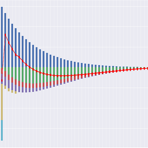
The by-policy projection of the Term_UK_S model.

The Space is parameterized by point_id, so Projection[1] is an ItemSpace projecting model point 1:

>>> Projection[1].result_cf()          # the worked example's anchor cell
>>> Projection.point_id = 3            # or switch the default

t counts policy months from issue, 0-based, as everywhere in lifelib: t = 0 is the issue month, t = proj_len() - 1 = term_mths() - 1 is the last, and the policy year containing month t is t // 12 + 1. The frame is range(proj_start(), proj_len()) — range(proj_len()) for a point projected from issue, opening at t = proj_start() = 12 x duration_inforce() for a point already in force. Month t runs from time t to time t + 1: pols_if(t) is the count at its start, premiums and maintenance expense fall at its start, claims and lapses at its end. There is nothing after the last month — cover ceases at the end of the term with no maturity value, no renewal and no conversion.

Input data

Inputs are external files: plain CSVs living in the model folder’s parent directory, products/term_assurance/, read at run time rather than stored inside the model. The model folder therefore holds nothing but formulas — no _data/, no IOSpec, no embedded values — so a diff of the model shows logic changes only, and an input can be edited or swapped without rewriting the model. This follows annuallife.TradLife_A; contrast basiclife.BasicTerm_S, which keeps its inputs inside the model through modelx’s IOSpec machinery.

The consequence worth knowing: the model is not portable on its own. Copying the Term_UK_S folder without its parent’s CSVs produces a model that reads and then fails on first evaluation.

Each table has a filename Reference and a reader Cells, both on Data, reached here through the data Reference:

Reference	Cells	File
model_point_file	data.model_point_table()	model_point_table.csv
mort_table_file	data.mort_table()	mort_table.csv
select_factor_file	data.select_factor_table()	select_factor_table.csv
lapse_table_file	data.lapse_table()	lapse_table.csv

Naming

Cells names follow lifelib’s basiclife.BasicTerm_S wherever that model has an analogue — pols_* for policy counts, plural nouns for cash flows, *_rate for annual rates and *_rate_mth for monthly ones, *_pp for per-policy amounts, claims(t, kind) with an uppercase kind string, pols_if_at(t, timing) for the within-month in-force reads. The technical notes use compact actuarial symbols instead. The mapping is:

Notes symbol	Cells	Meaning
shape	shape()	level / decreasing / fib
x	age_at_entry(life)	Issue age (ANB), life 1 or 2
x + duration(t)	age(t, life)	Attained age in month t
(none)	sex(life), smoker(life)	Rating factors of each life
n	policy_term()	Term in years
N = 12n	term_mths()	Term in months, = proj_len()
(none)	proj_len()	Months projected; last t is N-1
(none)	proj_start()	First projected t
(none)	duration_inforce()	Years elapsed at projection start
k, duration_mth(t)	duration_mth(t)	Months elapsed since entry, = t
(none)	duration(t)	Completed years since entry, t//12
(none)	policy_year(t)	Contractual policy year, t//12 + 1
SA0	sum_assured()	Initial sum assured
I	fib_income()	FIB income per month
j	sched_rate()	Decreasing schedule rate p.a.
j_m	sched_rate_mth()	(1+j)^(1/12) - 1
B(k)	benefit_sched(k)	Decreasing benefit after k months
DB(t)	benefit_pp(t)	Death/TI benefit per policy
idx(t)	idx_factor(t)	Cover indexation factor
idx_p(t)	idx_prem_factor(t)	Premium indexation factor
(RPI scenario)	rpi_rate	Flat RPI assumption, 3%
P_m	premium_mth_pp()	Monthly premium at outset
P_m x idx_p(t)	premium_pp(t)	Premium due in month t
(mode)	premium_mode()	monthly or annual collection
(table)	mort_rate_base(t, life)	Table rate before adjustment
(select)	select_factor(t)	Select-duration factor
(proxy scaling)	mort_scale	“00” to “16” Series factor
(none)	mort_rate_life(t, life)	Per-life annual rate
q(t), q_joint	mort_rate(t)	Annual policy decrement, incl. TI
q_m(t)	mort_rate_mth(t)	Monthly policy decrement
(none)	mort_basis()	applied or select run
lambda	sel_lapse_lambda	Selective-lapsation loading
w_ref	sel_lapse_ref	Selective-lapsation threshold
w_cum(t)	lapse_cum(t)	Cumulative lapse proportion
(none)	sel_lapse_factor(t)	Mortality loading on persisters
(table)	lapse_rate_base(t)	Table annual lapse rate
M_reb(t)	rebroke_factor(t)	Rebroking multiplier
w(t)	lapse_rate(t)	Annual lapse rate in month t
w_m(t)	lapse_rate_mth(t)	Monthly lapse rate
l(t)	pols_if(t)	In force at the start of month t
l(t)(1-q_m), l(t+1)	pols_if_at(t, timing)	BEF_DECR / BEF_LAPSE / AFT_DECR
D(t)	pols_death(t)	Expected death/TI claims
(none)	pols_lapse(t)	Lapses at the end of month t
(none)	pols_maturity(t)	Expiries at the end of the term
(none)	pols_payer(t)	Policies actually paying premium
inc(t)	wop_inc_rate	WOP annual incidence rate
(recovery)	wop_rec_rate	WOP annual recovery rate
(deferred period)	wop_defer_mths	26 weeks, read as 6 months
(none)	wop_waived_frac(t)	Fraction with premiums waived
FIBcum(t)	fib_cum(t)	FIB streams already in payment
a(m)	annuity_certain_factor(m)	m-month annuity-certain factor
r_c	fib_commute_disc_rate	FIB commutation rate, 3%
CV(k)	fib_commute_pp(t)	Commuted value of one stream
(take-up)	fib_commute_rate()	Proportion of FIB claims commuted
P_m x idx_p x l	premiums(t)	Premium income
DB(t) x D(t), Claims_fib	claims(t, kind)	Benefit outgo by kind
ec x D(t)	claim_expenses(t)	Claim expense outgo
E0, e(t)	expenses(t)	Acquisition + maintenance
(none)	inflation_factor(t)	Expense inflation factor
c0	comm_init_pp()	Initial commission per policy
c_r	comm_renewal_rate	Renewal commission rate
(clawback)	comm_clawback(t)	Commission recovered on lapse
c0, c_r x premiums	commissions(t)	Commission outgo, net
CF(t)	net_cf(t)	Net cash flow, income positive

Five names needed care.

The notes use q(t) both for the per-life table rate and for the decrement actually applied to the policy, which on a joint first-death policy is 1 - (1-q_1)(1-q_2). mort_rate_life() is the per-life rate and mort_rate() the policy decrement, so the joint combination has somewhere to live and the single-life case collapses to the same number.

q(t) and w(t) are annual rates in the notes and stay annual here, with mort_rate_mth() and lapse_rate_mth() carrying the monthly conversions 1 - (1 - q)^(1/12) and 1 - (1 - w)^(1/12). That is the library-wide split — a bare *_rate is the annual rate everywhere, and only *_rate_mth is monthly — and it is what lets the assumption tables stay in the annual units they are quoted in.

w(t) is the lapse rate and w_cum(t) the cumulative lapse proportion that drives the selective-lapsation loading on mortality. Spelling them lapse_rate and lapse_cum keeps the second from reading as a running total of the first, which it is not: it is a proportion of the original cohort, and the loading it feeds moves claims, not lapses.

E0 and e(t) are the acquisition and maintenance expenses; both are inside expenses(), which is the library-wide name, with the claim expense ec x D(t) kept out of it under claim_expenses() because the notes’ worked-example table prints the two as separate columns.

pols_maturity has no symbol in the notes at all. The notes give the roll-forward as l(t+1) = l(t)(1-q_m)(1-w_m) and, separately, terminate everything at month N. Those do not reconcile in the final month: its survivors neither die nor lapse — their cover simply runs out — so without a term for that the roll-forward appears to lose lives with no cause. pols_maturity() names it, zero in every month but the last, so that

pols_if(t) - pols_if(t+1) = pols_death(t) + pols_lapse(t) + pols_maturity(t)

holds for every t; check_pols_roll_fwd() asserts it. It is bookkeeping determined by the notes’ own rules, not an added assumption, and the name follows BasicTerm_S.pols_maturity. Note that it is not a maturity benefit: the amount paid is nil.

The monthly grid, and what it removes

The notes take an annual grid as their base and a monthly one as its arbiter: the annual grid has to read the decreasing shape’s monthly step-down as a mid-year balance B(12t + 6), to annualize the premium and carry it in advance with no allowance for a mid-year death or lapse, and to round the family income benefit’s instalment count to six in the year of death and twelve thereafter. The notes are explicit that the first two are an offsetting pair of biases and that the monthly grid is what settles them.

This model is that monthly grid, so none of those approximations is here. The decreasing benefit is the exact balance benefit_sched() (t) of the month the claim falls in; the premium is the contractual monthly premium P_m, collected in the months it is actually due, and it stops the month the policy leaves; family income benefit instalments are counted one by one. What the annual grid could only offset, the monthly grid simply does not incur.

Two further things follow. premium_mode is no longer inert: a policy paying annually is charged 12 P_m in the first month of each policy year and nothing in the other eleven, which is a real difference in the timing of income on a grid that can see it. And the waiver of premium rider’s 26-week deferred period, which the annual grid could only read as “incidence in year t, waiver from year t + 1”, is carried explicitly as wop_defer_mths = 6 months.

The assumption tables are unchanged and stay in the annual units they are quoted in: mort_table.csv is an annual rate by attained age, lapse_table.csv an annual rate by policy year. mort_rate_mth() and lapse_rate_mth() convert them with 1 - (1 - r)^(1/12) [std], the notes’ own monthly-grid convention, so twelve months compound back to the annual rate exactly. Both are stepped by policy year, not by month: the attained age advances on the policy anniversary, which is what an age-nearest- birthday basis means, and the lapse table is keyed by the contractual policy year.

No tail states

This is the structural difference from Term_US_S, and the notes list importing a U.S.-style post-level-term tail as a modelling pitfall. A UK term policy expires at the end of month N - 1: there is no jump to ART rates, no post-level-term shock lapse, no mortality deterioration factor and no conversion option, so none of those cells exist here. What does exist and has no U.S. analogue is the family income benefit ledger below.

Terminal illness is not an extra benefit

Terminal illness is a 100% acceleration of the death benefit under a two-limb 12-month definition, not an additional cover: one decrement, one payment. Adding a separate terminal-illness decrement double-counts claims, which is the notes’ first-listed pitfall, and the CMI “16” Series assured lives tables already include terminal illness. So mort_rate is the combined death-and-terminal-illness rate and there is no ti_rate anywhere in the model. The acceleration shifts payment earlier by up to twelve months; modelling that shift would need a separate terminal-illness diagnosis basis, which the subscriber-restricted tables do not provide, so it is left out on the monthly grid as it was on the annual one [std].

The family income benefit ledger

A death in month k on the fib shape triggers N - k monthly instalments of I, in arrears, ending at month N. The instalments are an annuity-certain: once the claim is admitted they run to the end of the term regardless of any life, so the in-payment stream is decremented by neither mortality nor lapse. Only new claims carry l(t). Omitting the ledger — paying only the instalment falling in the month of death — understates the liability by up to N - 1 months of income, and the notes list it as a pitfall.

fib_cum() is that ledger: the expected number of streams already in payment at the start of month t, sum of D(s) for s < t. Each stream pays one instalment at the end of each month from the month of death onwards, so

claims(t, “FIB”) = I x [D(t) + FIBcum(t)]

and the whole stream for a death in month s totals N - s instalments, which is the notes’ count at the exact death month with no rounding — the six-and-twelve bookkeeping the annual grid needed is gone. check_fib_ledger() rebuilds the month’s instalment count from the death vector, with no reference to the recursion, and asserts the two agree in every projected month.

The optional commutation module replaces a proportion fib_commute_rate() of the streams with a lump sum, the present value of the remaining instalments at the [std] snapshot rate r_c = 3%. Contractually the insurer reduces the sum of the remaining instalments “fairly and reasonably” and no insurer publishes the basis, so the rate is a standardization; base take-up is zero and model point 4 exercises the other extreme.

Two mortality bases: applied and select

UK assured-lives tables are select tables — TMNL16/TFNL16 have a 5-year select period, AM92 a 2-year one — so the mortality interface has to accept a rate that depends on duration since entry as well as attained age. But the notes’ worked example is quoted as three applied rates, q(0) = 0.00055, q(1) = 0.00060, q(2) = 0.00065, described as illustrative values in the shape of a non-smoker temporary assurance table and explicitly not taken from any CMI table. Three numbers rising at 9% a year are not consistent with a graduated select structure, where the wearing-off of selection alone moves the rate faster than that. Forcing them onto one would mean either a back-solved ultimate curve that is nearly flat at ages 35-37 or shipped cells that deviate from the notes. Both are shipped instead, and which applies is a model point column:

mort_basis = "applied" [std]: mort_table.csv is read as the annual rate actually applied: no select factor, no proxy scaling. Model points 1-6 and 8; point 1 is the anchor cell and reproduces the worked example to the penny.
mort_basis = "select": the same table is read as an ultimate basis and multiplied by select_factor() and by mort_scale, the notes’ [std] 75% proxy for improvement from the public “00” Series era to the 16-Series era. Model point 7. This is the shape a production run takes once licensed tables are dropped in — replacing the two CSVs changes the basis with no formula change.

Both are standardizations. The shipped table is a [std] construction throughout: the M/N cells at ages 35-37 are the notes’ illustrative vector, and every other cell is a 9% p.a. geometric extension in age with a 2.2 smoker and a 0.70 female factor, each row tagged in the file’s provenance column. It is not a published table and no conclusion about UK mortality should be drawn from it.

Modules that are off in the base run

Four of the notes’ optional constructions are implemented and switched off, so that the base run reproduces the worked example while the machinery stays visible and testable:

Selective lapsation, q_eff = q (1 + lambda max(0, w_cum - w_ref)), with lambda = 0. Healthier lives lapse, so persisters are progressively impaired; the notes rate it the third-largest lever on a long-term block.
Rebroking, M_reb = min(2, max(1, P_inforce / P_market)) on the lapse rate, with premium_market_ratio at 1. Guaranteed premiums rule out premium-shock lapse, so falling market rates for the attained age are the economic driver instead. The Reference is a flat scalar, so the multiplier is level in t; a market premium path would be another input table.
Commission clawback on lapse inside the clawback window, linear in months in force, with clawback_mths at 0. Set it to 48 for the notes’ four-year rule. The months in force at the end of month t are t + 1 exactly, so on this grid the linear run-off is read month by month rather than in twelve-month jumps.
Waiver of premium, a two-state incidence/recovery chain on the premium-paying population, with wop false on every model point but 7. Both its incidence basis and its extra premium are [std] placeholders: no public UK incidence basis for the work-tasks definitions exists in the sources. The 26-week deferred period is carried as wop_defer_mths = 6 months between incidence and the first waived premium [std], and mortality and lapse are assumed independent of the waiver state [std], which is what lets the waived population be carried as a fraction rather than as a separate decrement.

Sign convention

The notes’ CF(t) is already income positive — “+ = inflow” — which is the library-wide sign of net_cf(), so unlike the whole life and payout annuity models there is no liability_cf companion to publish: one stream, one sign, one name.

Lapse pays nothing

There is no surrender value and no paid-up value at any duration, so a lapse is a pure decrement: it moves pols_if and pays nothing. claims(t, "LAPSE") exists and returns zero, and result_cf() carries the zero column, because the notes list a non-zero lapse row as a pitfall imported from US models with cash surrender values — a column of zeros states the product fact where a missing column would only hide it.

Cells Descriptions#

model_point()[source]#: The selected model point as a Series.

shape()[source]#: The benefit shape: level, decreasing or fib [S1][S2][S6][S8].

is_joint()[source]#

True when the policy covers two lives on a first-death basis.

The policy pays once and ends; separation and replacement options create new policies and are out of scope [std scope].

age_at_entry(life=1)[source]#

x: the issue age (ANB) of the first (life = 1) or second life.

Age nearest birthday at entry, plus a curtate policy year [std]: the fetched product documents state no age basis, and the UK assured lives tables are select tables indexed that way.

sex(life=1)[source]#: The sex (M / F) of the first or second life.

smoker(life=1)[source]#: The smoker status (N / S) of the first or second life.

policy_term()[source]#: n: the term in years; 1-50 level, 5-50 decreasing, 5-40 FIB [S1][S6][S8].

sum_assured()[source]#: SA0: the initial sum assured of the level and decreasing shapes [S1][S6].

fib_income()[source]#: I: the family income benefit, per month, on the fib shape [S2][S6][S8].

sched_rate()[source]#

j: the decreasing shape’s schedule rate p.a. [std], 6% on the shipped points.

Contractual, not experience: the client selects it at outset and the benefit amortizes at it whatever happens to interest rates [S1][S6][S8]. The risk it carries is therefore specification error - mis-implementing the amortization or the monthly convention - rather than assumption error.

indexation()[source]#

Whether the RPI indexation option is elected [S1][S2][S6][S7].

Restricted to the level shape [std scope]: no fetched insurer offers indexed decreasing cover, and the notes do not combine indexation with the FIB schedule either.

wop()[source]#: Whether the waiver of premium rider is in force [S1]; false in the base run.

premium_mth_pp()[source]#

P_m: the guaranteed monthly premium per policy [std].

A pure modelling value. No UK insurer publishes premium rate tables - pricing is quote-driven and only the £5/month minimum is public [S5] - so any reference premium basis is constructed rather than observed. It is guaranteed level for the full term [S2][S6][S9], which is what puts every month of premium inside the Solvency UK contract boundary [R3].

premium_mode()[source]#

Monthly or annual premium collection.

Live on this grid, unlike the annual one, which annualized either way. A monthly payer is charged P_m in every month; an annual payer is charged 12 P_m in the first month of each policy year and nothing in the other eleven. The amount collected over a policy year is the same and only its timing differs, so the difference is small and one-signed: the annual payer’s income arrives earlier and is collected in full from a life that may leave during the year. No premium discount for annual collection is modelled [std]; UK protection pricing is quote-driven and no published scale exists.

mort_basis()[source]#

Whether the mortality table is read as the applied rate or as an ultimate one.

applied [std] takes mort_table.csv as the annual rate actually applied, which is how the notes quote their illustrative worked-example vector; select multiplies it by select_factor() and by mort_scale, the notes’ proxy for the unavailable subscriber tables. See the Space docstring for why both are shipped.

pols_if_init()[source]#: Initial number of policies in force; 1.0 on a single-policy model point.

duration_inforce()[source]#

Completed policy years already elapsed when the projection starts; 0 at issue.

A policy attribute, carried on the model point in the units a contract speaks in, and converted to the grid’s months by proj_start().

fib_commute_rate()[source]#

The proportion of FIB claims commuted to a lump sum [std]; 0 in the base run.

The insurer may replace the remaining instalments with a lump sum determined “fairly and reasonably” [S6][S8]; no insurer publishes the basis, so both the take-up and the discount rate fib_commute_disc_rate are standardizations.

proj_start()[source]#

The first projected month: 12 x duration_inforce(), the elapsed months.

0 at issue, so the acquisition expense and the initial commission fall inside the projection; an in-force model point starts on the anniversary that opens its next policy year and never sees either.

proj_len()[source]#

The number of policy months counted from issue: 12n, exactly term_mths().

The exclusive end of the frame, which runs t = proj_start(), ..., proj_len() - 1 - range(proj_len()) for a point projected from issue. Cover ceases at the end of the term with no maturity value, no renewal and no conversion [S1][S2][S6][S8][R8], so the horizon is N = 12n months and there is nothing after t = N - 1 - the structural contrast with Term_US_S, which runs on to attained age 95.

term_mths()[source]#: N = 12n: the term in months, the horizon of the benefit schedules and the frame.

duration(t)[source]#

Completed years since entry at the start of month t: t // 12, 0 in the first.

The select duration, which is what the UK assured lives tables are indexed by alongside attained age. t counts from issue for every model point, so an in-force point’s duration is measured from entry, not from the projection start.

duration_mth(t)[source]#

Months elapsed from issue at the start of month t; equal to t.

The notes’ benefit-schedule index k. t is 0-based and counts from issue, so the identity is trivial - the cells exists so the monthly models in this library share one vocabulary.

policy_year(t)[source]#

The contractual policy year containing month t: the 1-based label t // 12 + 1.

Used only where a 1-based schedule is looked up - the lapse table’s policy_year key. Never the index of anything in the projection.

age(t, life=1)[source]#

The attained age (ANB) of life in month t: x + duration(t).

Advances on the policy anniversary rather than monthly, which is what an age-nearest-birthday basis means and how the mortality table is entered.

select_factor(t)[source]#

The select-duration factor applying in month t [std].

A 5-year select period, the structure of TMNL16/TFNL16 [R12], with the factor grading from 0.55 at duration 0 to 1.00 at and beyond select_period. Stepped by completed policy year, like the table it multiplies. Read only on the select mortality basis; the applied basis takes the table as it stands. The values are a standardization - the real tables are subscriber-only [R11] - and a licensed basis drops in by replacing the CSV.

mort_rate_base(t, life=1)[source]#

The annual mortality table rate for life at its attained age in month t.

Includes terminal illness, which is an acceleration of the death benefit rather than a separate cover [S1][S6][S8]; the 16-Series tables the shipped table proxies are graduated on that basis [R10].

mort_rate_life(t, life=1)[source]#

The annual mortality (incl. TI) rate applied to life in month t.

The table rate, then on the select basis the select factor and the [std] 75% proxy scaling, then the selective-lapsation loading. Capped at 1.

mort_rate(t)[source]#

q(t): the annual mortality (incl. TI) decrement of the policy in month t.

The single life’s rate on a single-life policy. On a joint first-death policy it is the joint decrement 1 - (1 - q_1)(1 - q_2) [std] on one policy, which pays once and ends [S1][S6]; modelling the two lives as separate policies would pay twice. mort_rate_mth() is what the projection actually decrements by.

mort_rate_mth(t)[source]#

q_m(t) = 1 - (1 - q(t))^(1/12): the monthly death and TI decrement [std].

The notes’ own monthly-grid conversion, so the twelve months of a policy year compound back to that year’s annual rate exactly. The nominal alternative q/12 does not: twelve months of it leave (1 - q/12)^12 > 1 - q, so it understates the decrement, by more the larger the rate. The effective monthly rate is therefore always a little above q/12.

lapse_cum(t)[source]#

w_cum(t): the cumulative lapse proportion of the original cohort before month t.

A proportion of pols_if_init(), not a running total of lapse_rate(), and it drives a loading on mortality rather than on lapse. Zero in the first projected month.

sel_lapse_factor(t)[source]#

The selective-lapsation loading on mortality in month t [std].

1 + lambda max(0, w_cum(t) - w_ref). Lapsers are healthier than persisters, so a block that has already shed a large proportion of its lives carries impaired mortality on the remainder - guaranteed premiums plus healthy-life rebroking make this a structural feature of UK term rather than an incidental one. Off in the base run (sel_lapse_lambda = 0), where it returns 1 in every month.

lapse_rate_base(t)[source]#

The table annual lapse rate in month t [std], before any rebroking.

10 / 8 / 7 / 5 / 6 / 4 percent, anchored to the FCA’s 5% average in-force lapse rate for pure protection and to the spike pattern just after the two- and four-year commission clawback periods end [R9]. A full duration curve is not public and the levels are standardized calibrations. The table is keyed by the contractual 1-based policy year, read at policy_year() (t) = t // 12 + 1; policy years beyond the table take its last row.

rebroke_factor(t)[source]#

M_reb(t): the rebroking multiplier on the lapse rate [std]; 1 in the base run.

min(rebroke_cap, max(1, P_inforce / P_market)). Premiums are guaranteed, so there is no premium-shock lapse to model; the economic driver is rebroking when market premiums for the attained age fall below the in-force premium. premium_market_ratio is a flat scalar, so the multiplier is level in t - a market premium path would be another input table.

lapse_rate(t)[source]#

w(t): the annual lapse rate applying in month t.

The table rate times the rebroking multiplier, capped at 1. A lapse pays nothing: there is no surrender or paid-up value at any duration [S1][S6][S8][R8].

lapse_rate_mth(t)[source]#

w_m(t) = 1 - (1 - w(t))^(1/12): the monthly lapse rate [std].

The notes’ monthly-grid conversion, so twelve months of a policy year compound back to that year’s table rate exactly. As with mort_rate_mth(), a nominal w/12 would understate the decrement; the gap is wider here because the lapse rates are an order of magnitude larger than the mortality ones.

pols_if(t)[source]#

l(t): the number of policies in force at the start of month t.

pols_if_init() in the first projected month t = proj_start() (l(0) = 1 at issue), then the notes’ monthly recursion l(t+1) = l(t)(1 - q_m(t))(1 - w_m(t)). This is the weight on every cash flow of the same result_cf() row. Zero outside proj_start() .. proj_len() - 1: the cover has not started or has expired.

pols_if_at(t, timing)[source]#

The number of policies in force at a point inside month t.

"BEF_DECR": l(t), the start of the month, before any decrement; the same number as pols_if() and the weight on that month’s cash flows.
"BEF_LAPSE": after deaths, before lapses - the notes’ processing order is death before lapse [std order], so this is the population lapses are taken from.
"AFT_DECR": l(t+1), the end-of-month state: what is left once the month’s deaths and lapses are taken, and zero from the final month t = proj_len() - 1 on because the cover expires at its end.

pols_death(t)[source]#

D(t) = l(t) q_m(t): expected death and terminal illness claims in month t.

One decrement covering both: terminal illness accelerates the death benefit rather than adding to it [S1][S6][S8].

pols_lapse(t)[source]#

Lapses at the end of month t, taken from the survivors of mortality.

Pays nothing - there is no surrender value [S6][R8] - so this moves pols_if() and nothing else.

pols_maturity(t)[source]#

Policies whose cover expires at the end of the term; zero in every other month.

Non-zero only in the final month t = proj_len() - 1. Not a decrement and not a benefit - the contract simply runs out, with no maturity value [S1][S2][S6][S8][R8] - but needed for the in-force roll-forward to close; see the Space docstring and check_pols_roll_fwd().

wop_waived_frac(t)[source]#

The fraction of in-force policies with premiums waived at the start of month t.

A two-state incidence/recovery chain at monthly rates [std], with the 26-week deferred period [S1] carried explicitly as wop_defer_mths months between incidence and the first waived premium:

u(t+1) = u(t)(1 - rec_m) + inc_m (1 - u(t - defer)) (1 - rec_m)^defer

The entrants of month t + 1 are the lives who became incapacitated defer months earlier and have not recovered since. That is what the monthly grid buys here: the annual grid could only read the deferred period as “incidence in year t, waiver from year t + 1”, rounding 26 weeks to twelve months.

Both rates are placeholders: no public UK incidence basis for the waiver work-tasks definitions appears in the fetched sources. Mortality and lapse are assumed independent of the waiver state [std] - which is what lets the waived population be carried as a fraction of the in-force rather than as its own decrement. Zero unless the rider is in force.

wop_inc_rate_mth()[source]#: inc_m: the monthly waiver incidence rate, 1 - (1 - inc)^(1/12) [std].

wop_rec_rate_mth()[source]#: rec_m: the monthly waiver recovery rate, 1 - (1 - rec)^(1/12) [std].

pols_payer(t)[source]#

The number of in-force policies actually paying premium in month t.

l(t) less the waived fraction. Equal to pols_if() unless the waiver of premium rider is in force.

idx_increase()[source]#

The cover increase offered at each anniversary under the indexation option.

min(max(RPI, 0), 10%) [S1][S2][S6][S7], times idx_accept_rate. The notes’ base run is deterministic and always accepts, which is what the shipped idx_accept_rate = 1 means; their 80% take-up [std] would be a mixture of paths, and scaling the increase instead is a deterministic approximation to it.

One consequence worth stating: with acceptance certain, the rule removing the option after three consecutive declines [S1][S6] (two at one insurer [S8]) is never reached, so it is not implemented.

idx_factor(t)[source]#

idx(t): the cumulative cover indexation factor in month t.

Steps on the policy anniversary and is level through the policy year, because the increase is offered at an anniversary and not monthly: 1 in the first projected policy year, then one factor of 1 + idx_increase() per anniversary passed. 1 whenever the option is not elected.

idx_prem_factor(t)[source]#

idx_p(t): the cumulative premium indexation factor in month t.

The premium rises by min(1.5 x increase, 15%) for a cover increase of increase [S1][S2][S6], on the same anniversary step as the cover factor. The 1.5 multiplier is what makes an accepted increase premium-margin-accretive if mortality is proportional to cover - and what reverses the sign of that conclusion if acceptance is selective, impaired lives accepting while healthy ones decline [std] concern. No public take-up data exists.

premium_pp(t)[source]#

P_m idx_p(t): the gross premium per policy due in month t.

The contractual monthly premium on a monthly payer, and 12 P_m in the first month of each policy year and nil in the rest on an annual one - the timing difference the annual grid could not see. Indexed if the option is elected, and loaded by wop_prem_loading where the waiver rider is in force - a [std] placeholder, since the rider’s extra premium is not published either.

premiums(t)[source]#

Premium income at the start of month t, an inflow.

Carried on pols_payer(), never on the FIB ledger: premiums stop at death while family income benefit instalments continue. Collected only from the policies still in force at the start of the month, so the annual grid’s overstatement - a full year’s premium taken from a life that leaves mid-year - does not arise.

sched_rate_mth()[source]#

j_m = (1+j)^(1/12) - 1: the decreasing schedule’s monthly rate [std].

The effective convention, not a nominal j/12. The two give slightly different schedules, so the convention has to be stated; benefit_sched(60) = £134,588 on the anchor cell is the notes’ validation anchor for an implementation.

benefit_sched(k)[source]#

B(k): the decreasing shape’s benefit after k months [S1][S6][S8].

SA0 [(1+j_m)^N - (1+j_m)^k] / [(1+j_m)^N - 1], a mortgage-style amortization from B(0) = SA0 to B(N) = 0. A zero schedule rate degenerates to straight line, which the closed form cannot express.

annuity_certain_factor(m)[source]#

a(m): the m-month annuity-certain factor at the FIB commutation rate [std].

[1 - (1+r_c)^(-m/12)] / [(1+r_c)^(1/12) - 1], instalments in arrears. Used only by the commutation module.

fib_commute_pp(t)[source]#

CV: the commuted value of one FIB stream arising from a death in month t [std].

I a(N - t) at the exact death month k = t, so it falls to zero as the term runs out. The annual grid had to place the death at mid-year, k = 12t + 6; this grid knows the month. Zero on the level and decreasing shapes.

benefit_pp(t)[source]#

DB(t): the death and terminal illness benefit per policy in month t.

Level: SA0 idx(t). Decreasing: the exact schedule balance B(t), the outstanding amount through the month the claim falls in - the annual grid’s mid-year reading B(12t + 6) was an approximation to this and is gone. FIB: the commuted value of the instalment stream, which is what a commuted claim pays; an uncommuted FIB claim has no lump sum at all and goes through claims(t, "FIB") instead.

fib_cum(t)[source]#

FIBcum(t): the expected FIB streams already in payment at the start of month t.

sum of D(s) for s < t. Not decremented by mortality or lapse: once a claim is admitted the instalments are an annuity-certain to the end of the term whatever happens to any life [S6][S8]. Only new claims carry l(t).

claims(t, kind=None)[source]#

Benefit outgo in month t, by kind; the total when kind is omitted.

"DEATH": the lump sum paid at the end of the month of death: DB(t) D(t) on the level and decreasing shapes, and on the fib shape only the commuted proportion of the streams.
"FIB": the family income benefit instalments falling in month t, I [D(t) + FIBcum(t)] net of the commuted proportion - one instalment for every stream in payment, the month’s new claims included, since the instalments are in arrears from the month of death. Zero on the other two shapes.
"LAPSE": zero, always. There is no surrender or paid-up value at any duration [S1][S6][S8][R8]; the kind exists so that the zero is stated rather than left to inference. See the Space docstring.

claim_expenses(t)[source]#

ec D(t): the claim handling expense on the month’s death and TI claims [std].

£250 per claim, uninflated. Kept out of expenses() because the notes’ worked example prints the two as separate columns.

inflation_factor(t)[source]#

The expense inflation factor in month t: (1 + pi)^duration(t) [std].

Steps on the policy anniversary rather than monthly, which is how the notes write it: e(t) = 30 x 1.03^t with t the policy year. 1 in the first policy year.

expenses(t)[source]#

E0 and e(t): acquisition and inflating maintenance expense in month t [std].

£150 per policy at issue (t = 0), then £30 per policy per year - a twelfth of it each month - inflating at 3% on each anniversary, both at the start of the month. An in-force model point starts after t = 0 and never sees the acquisition charge. Premiums as low as £5/month against a £30 annual maintenance expense make this assumption solvency-relevant on small-sum-assured blocks, which is why the notes rate expense inflation a first-order lever despite its size.

comm_init_pp()[source]#

c0: initial commission per policy issued [std].

150% of the annualized premium of the first policy year, 12 P_m on an unindexed point, paid upfront at issue. Roughly 96% of protection commission is paid upfront [R9], which with the acquisition expense is what produces the deep first-month new business strain in the worked example.

comm_clawback(t)[source]#

Initial commission recovered on lapses inside the clawback window [std].

c0 (clawback_mths - (t+1))/clawback_mths per lapsed policy, linear in months in force: a lapse at the end of month t has t + 1 months in force, which this grid counts exactly where the annual one could only step twelve at a time. Off in the base run (clawback_mths is 0); set it to 48 for the notes’ four-year rule. Clawback periods of two to four years are evidenced [R9]; the linear formula is a standardization. Inside the window it reverses the sign of the early-lapse sensitivity, which is the point of carrying it.

commissions(t)[source]#

Commission outgo in month t [std], net of any clawback recovered.

The initial commission at issue (t = 0), then 2.5% of premium income from the second policy year (t >= 12). Both are levels chosen for the reference implementation; only the upfront pattern is evidenced [R9].

net_cf(t)[source]#

CF(t): the net cash flow of month t, income positive.

Premiums less death and terminal illness claims, claim expense, maintenance and acquisition expense and commission. The notes’ own sign - they write + = inflow - which is also the library-wide convention, so unlike the whole life and payout annuity models there is no outgo-positive liability_cf companion to publish.

The shape to expect on guaranteed term is a deep new business strain in the first month (t = 0), upfront commission and acquisition expense against a single month’s premium, then thin positive margins: the level premium prefunds rising mortality cost, so early lapses forfeit margin to the insurer and late ones relieve it.

check_pols_roll_fwd_resid(t)[source]#

The in-force roll-forward residual in month t; zero everywhere.

pols_if(t) - pols_if(t+1) - deaths - lapses - expiries. Expiries are non-zero only in the final month t = proj_len() - 1, where the survivors neither die nor lapse: their cover runs out. Without that term the last month appears to lose lives with no cause.

check_pols_roll_fwd()[source]#

True when the in-force roll-forward closes in every projected policy month.

The library-wide form of a roll-forward check: no argument, one bool over all t, so one test can call it across every model. check_pols_roll_fwd_resid() gives the signed residual of the month that failed. The tolerance scales with pols_if_init(), since the residual accumulates rounding on that many policies.

check_fib_ledger_resid(t)[source]#

The family income benefit ledger residual in month t; zero everywhere.

claims() (t, "FIB") less an independent rebuild of the same figure: one instalment for every death in month t or any earlier month, summed straight off the death vector with no reference to the fib_cum() recursion. A ledger that was decremented by mortality or lapse - the notes’ pitfall - or one that paid only the month-of-death instalment would show up here. Zero by definition on the level and decreasing shapes, which have no ledger.

check_fib_ledger()[source]#

True when the family income benefit ledger closes in every projected month.

No argument, one bool over all t, the library-wide shape of a check_* cells; check_fib_ledger_resid() gives the signed residual of the month that failed.

result_cf()[source]#

Result table of cashflows, indexed by policy month t.

One row per month t = proj_start(), ..., proj_len() - 1 - proj_len() rows for a point projected from issue. pols_if is the start-of-month count, which is the weight applied to every cash flow on the same row. net_cf carries the notes’ own income-positive sign. claims_lapse is a column of zeros by product design - there is no surrender value - and is published rather than dropped; see the Space docstring.

result_pols()[source]#

Result table of policy counts and decrement rates, indexed by policy month t.

The same rows as result_cf(): t = proj_start(), ..., proj_len() - 1. The two rate columns are the monthly decrements the projection actually applies; the annual rates they come from are mort_rate() and lapse_rate().