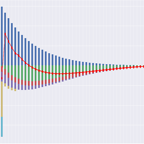
The Projection Space

The by-contract projection of the PA_UK_S model.

The Space is parameterized by point_id, so Projection[1] is an ItemSpace projecting model point 1:

>>> Projection[1].result_cf()          # the worked-example scenario
>>> Projection.point_id = 2            # the same contract, probability-weighted

t counts months from the annuity start date, 0-based: t = 0 is the first projected month and the frame is t = 0, 1, ..., proj_len() - 1. Month t runs from time t to time t + 1, so a flow of month t reads a state variable at t for its opening value and at t + 1 for its closing one, and the policy year containing month t is t // 12 + 1.

The state cells are indexed by a time point k, k = 0 at the start date: lives_if(), lives_if_last(), cum_annuity_pp() and vp_balance(). That index does not move with the frame — the annuitant who dies in month 16 is alive at time 16 and dead at time 17 — and every recursion’s base case sits at k = 0 (lives_if(0, life) = 1, cum_annuity_pp(0, kind) = 0). rpi_index() and rpi_peak() are indexed on a different scale again — an anniversary count, one step per policy year, 0 at outset, so rpi_index(1) is the reference level one year in — and it too is unmoved by the frame. Everything else — rates, factors, payment months, cash flows — is indexed by the month it belongs to.

Input data

Inputs are external files: plain CSVs living in the model folder’s parent directory, products/pension_annuity/, read at run time rather than stored inside the model. The model folder therefore holds nothing but formulas — no _data/, no IOSpec, no embedded values — so a diff of the model shows logic changes only, and an input can be edited or swapped without rewriting the model. This follows annuallife.TradLife_A; contrast basiclife.BasicTerm_S, which keeps its inputs inside the model through modelx’s IOSpec machinery.

The consequence worth knowing: the model is not portable on its own. Copying the PA_UK_S folder without its parent’s CSVs produces a model that reads and then fails on first evaluation.

Each table has a filename Reference and a reader Cells, both on Data, reached here through the data Reference:

Reference	Cells	File
model_point_file	data.model_point_table()	model_point_table.csv
mort_table_file	data.mort_table()	mort_table.csv

Naming

Cells names follow lifelib’s basiclife.BasicTerm_S and savings.CashValue_SE wherever those models have an analogue, and follow SPIA_US_S — this library’s U.S. payout chassis — wherever the two products share machinery, so that the same concept has the same name on both sides of the Atlantic. The technical notes use compact actuarial symbols instead. The mapping is:

Notes symbol	Cells	Meaning
t	(the cells argument)	Month from the start date, 0-based
k	(the cells argument)	Time point, k = 0 at the start date
a	(the cells argument)	Anniversary count, a = 0 at outset
y = t//12 + 1	policy_year(t)	Policy year containing month t
(none)	duration(t)	Completed policy years, y - 1
(none)	duration_mth(t)	Months elapsed at the start of month t
P	purchase_price()	Purchase price
x_a, x_d	age_at_entry(life)	Entry ages (ALB), life 1 or 2
(none)	age(t, life)	Attained age (ALB)
(none)	sex(life)	Sex of each covered life
theta_a, theta_d	rating_factor(life)	Enhanced/impaired multiplier
delta	dependant_pct()	Dependant’s percentage
(dependant_present)	is_joint()	Contract covers a dependant
overlap	overlap()	Dependant runs during guarantee
A(1)	annual_income_init()	Starting annualized income
A(y)	annual_income(y)	Annualized income in year y
g	escalation_rate()	Fixed escalation rate
escalation_type	escalation_type()	level / fixed / rpi_catchup / lpi5
I(a)	rpi_index(a)	RPI reference level at anniversary a
peak(a)	rpi_peak(a)	Running peak of I through anniversary a
m	payment_freq()	Payments per year
timing	payment_timing()	arrears or advance
T	is_payment_mth(t)	Month t is a payment date
s(t)	payment_surv_mth(t)	Time point survival is measured at
inst(t)	annuity_pp(t)	Scheduled instalment
n	guarantee_mths()	Guarantee period in months
C(t) = 1{t < n}	certain_floor(t)	Annuity-certain floor indicator
l_a(k), l_d(k)	lives_if(k, life)	Survival probability to time k
d_a(t), d_d(t)	lives_death(t, life)	Death density of month t
d_last(t)	lives_death_last(t)	Last-death density of month t
(none)	lives_if_last(k)	At least one covered life alive
max(C, l_a)	payment_factor(t)	Annuitant payment factor
(none)	payment_factor_life(t)	l_a alone, before the floor
w(t)	overlap_gate(t)	Dependant-stream availability
delta(1-l_a)l_d w	dependant_factor(t)	Dependant payment factor
G(k)	cum_annuity_pp(k, kind)	Scheduled instalments to time k
v	vp_pct()	Value-protection percentage
vp_basis	vp_basis()	first_death or last_survivor
VPbal(k)	vp_balance(k)	Value-protection balance at k
h(t)	mths_since_payment(t)	Complete months since last payment
proportion	proportion()	Proportionate final payment
(none)	next_payment_mth(t)	The next scheduled payment month
q_x (table)	mort_rate_base(t, life)	Base-table annual rate
alpha	annuitant_adj	Population-to-annuitant factor
f(x)	improve_rate(t, life)	Improvement rate at the age
(1-f)^(c-c0)	improve_factor(t, life)	Cumulative improvement factor
q_rated	mort_rate(t, life)	Annual rate after all factors
q_m	mort_rate_mth(t, life)	Monthly rate 1-(1-q)^(1/12)
(none)	mort_basis()	table or scenario run [std]
(none)	death_mth(life)	Scenario month of death [std]
omega	omega_age	Limiting age, 115
(stopping rule)	horizon_mths()	Months to the age stop rule
(none)	proj_len()	Projected months, the frame’s end
(none)	calendar_year(t)	Calendar year containing month t
IF(t)	pols_if(t)	Any payment obligation open
(none)	pols_if_init()	Contracts in force at the start
E[ANN(t)]	annuity_payments(t)	Expected annuity outgo
E[VP(t)]	claims(t, “VP”)	Value-protection lump sum
E[PROP(t)]	claims(t, “PROP”)	Proportionate final payment
E[EXP(t)]	expenses(t)	Maintenance expense
c_e, pi	expense_maint, inflation_rate	Expense level and inflation
CF(t)	liability_cf(t)	Total gross liability outgo
(none)	net_cf(t)	-liability_cf(t), insurer sign

Four names needed care.

G(t) is used for two different accumulations in the notes: the state variable table defines it as cumulative gross instalments scheduled, which is what the worked example’s G column prints, while the value-protection section says it accumulates instalments “while the annuitant is alive” on the first-death basis and “the dependant’s instalments too” on the last-survivor one. Those are different objects whenever the dependant’s stream is running, so cum_annuity_pp() takes a kind: "ANNUITANT" is the deterministic as-if-alive annuitant schedule that the first-death value-protection balance nets against, and "ALL" adds the expected dependant instalments and is the notes’ printed column.

l and L differ in the notes only by case, as in SPIA_US_S: survival probability against the payment factor. They become lives_if() and payment_factor_life(), with payment_factor() the certain-floored version.

w(t) is the overlap gate, not a lapse rate — there is no lapse on this product at all. It is spelled overlap_gate() so that nothing in the model reads as a decrement that is not one.

pols_if is not a policy count in the usual sense. It is the notes’ IF(t), the probability that any payment obligation remains — guarantee certain, annuitant alive, or dependant stream in payment — and it exists to carry the maintenance expense. The name is kept because it is what the rest of the library calls the expense weight.

Two mortality bases: table and scenario

The notes’ worked example is not a probability-weighted run. It is a scenario: “the annuitant dies in month 16; the dependant survives throughout”, evaluated at l_a = 0 from time 17 and l_d = 1 throughout. The rest of the notes projects on an expected basis. Both readings are shipped, and which one applies is a model point column — the same device SPIA_US_S uses for the same reason:

mort_basis = "table"

lives_if runs the generational recursion off the shipped mortality table and improvement scale. Model points 2, 5, 6, 7 and 8; point 2 is the worked configuration on this basis and is the run to read for a realistic cash flow shape.

mort_basis = "scenario" [std]

lives_if(k, life) is the deterministic step function 1{k <= death_mth(life)} — the life is alive up to the start of its death month and dead from the end of it — with a blank death_mth meaning the life survives the whole projection. Model points 1, 3, 4, 9 and 10, which reproduce the worked example and its variants exactly.

The scenario switch is a [std] modelling device, not a product feature; it exists because the notes’ verification anchor is a scenario and retuning assumptions to force a probability-weighted run onto it would be dishonest.

The guarantee is a floor, not a second stream

payment_factor(t) = max(certain_floor(t), payment_factor_life(t)) is the notes’ first-listed pitfall written as one line. During the guarantee period the full instalment is payable regardless of survival, escalating as if the annuitant were alive; an additive construction would pay 1 + l_a and silently double the guarantee.

The guarantee and value protection never coexist in the representative design — the contract offers one or the other, and check_guarantee_xor() asserts no model point carries both. An engine supporting the combinable variant would have to net guarantee payments off the value-protection balance or the death benefit is paid twice.

The overlap gate

overlap = False is the representative default and means the dependant’s stream starts only at the end of the guarantee period, not at the annuitant’s death. Applying the dependant’s percentage from the death date silently converts every without-overlap policy into the more expensive with-overlap form, which is the notes’ second-listed pitfall. Model points 3 and 4 are the same contract on either side of that switch, and their cash flows differ from month 17 to month 119.

Escalation, and the one path-dependent option

Four bases. level and fixed are self-explanatory; lpi5 is RPI floored at zero and capped at 5%; rpi_catchup is a ratchet: income is indexed to the running peak of the RPI reference index, so a fall in the index freezes income rather than reducing it, and later rises only bite once the index passes its previous peak. rpi_peak() carries that state across anniversaries. Resetting it each year turns the catch-up into a plain zero floor and overstates indexed income after a deflation-recovery path.

Under the deterministic 3% RPI assumption [std] the index is monotone, so the ratchet never binds and rpi_catchup degenerates to fixed 3% — model points 6 and 2 agree by construction. That is not an accident to be tidied away but the honest consequence of a deterministic inflation path: the zero floor, the ratchet and the LPI cap are all inflation options, and a deterministic path values them at intrinsic only. A market-consistent value needs stochastic inflation.

Escalation applies on the anniversary, not on payment dates: the year-2 rate does not reach the t = 11 arrears instalment, which accrued in year 1.

Value protection, and where the balance is measured

VP(t) = d(t) x max(0, v P - G(t)), the death benefit measured against instalments already paid. Two timing rules matter and both are the notes’ pitfalls:

• on arrears timing the balance is G(t), the balance at the start of the death month, because the instalment due at the end of it is never paid;

• on advance timing an instalment paid at the start of the death month has been paid, so in an advance payment month the balance is G(t + 1) — netting it, or the lump sum is overstated by one instalment.

On the first_death basis the death that triggers it is the annuitant’s and the balance nets the annuitant’s schedule alone. On last_survivor it is the last death, and the balance nets both streams — which, on a probability-weighted run, makes the balance an expected cumulative payment rather than a path-specific one. That approximation is stated here rather than hidden: it is exact in a scenario run, which is the basis the shipped last_survivor model point uses.

The contractual bound v + delta <= 1 on the first-death basis is asserted by check_vp_bound(); the worked configuration sits exactly on it.

There is no policyholder behaviour to model

No lapse decrement, no dynamic behaviour formulas, no surrender value at any time, no alteration of options and no premium flexibility. That is a cited product feature and the reason the liability is matching-adjustment eligible, and it is why this model has no lapse_rate of any kind. Behaviour enters only at outset, outside the projection, as basis-selection effects: voluntary annuitants self-select for longevity, which is the direction of the annuitant_adj factor below 1, and the enhanced-annuity market leaves standard-terms lives healthier on average, which is carried through rating_factor() rather than through any dynamic.

Sign convention

The notes define CF(t) as total gross liability outgo, which is liability_cf(). net_cf() is its negative, the library-wide income-positive convention, so a result_cf()["net_cf"] column can be summed or compared across every model in the library. Both are published as columns rather than one being made to stand for the other. There is no premium income in the projection at all: the purchase price is a pricing input paid at outset, before the first projected month, not a projected cash flow.

Cells Descriptions

model_point()

The selected model point as a Series.

purchase_price()

P: the amount applied to the annuity after any lump sum and adviser charges.

A pricing input paid at outset, before the first projected month, not a projected cash flow: the projection carries no premium income. It enters the projection only through value protection, where the guarantee is measured against it.

age_at_entry(life)

x: the entry age of the annuitant (life = 1) or dependant (life = 2).

Age last birthday, chosen to index the shipped single-year-of-age proxy table [std].

sex(life)

The sex (M / F) of the annuitant or dependant.

rating_factor(life)

theta: the enhanced or impaired mortality multiplier [std]; 1.0 standard.

q_rated = min(1, theta x q), the simplest overlay that reprices longevity without touching contract mechanics. Insurers’ real rating structures - postcode and condition-specific factors - are not public, and a rated-age offset is the equivalent form. Whole-market enhanced quoting is mandated at the point of sale, so lives remaining on standard terms are healthier on average; the model carries that through this multiplier rather than through any behavioural dynamic.

is_joint()

True when the contract carries a dependant’s income.

dependant_pct()

delta: the dependant’s percentage of the income; zero on a single-life contract.

overlap()

Whether the dependant’s stream runs during the remaining guarantee period.

False is the representative default and means the stream starts at the end of the guarantee, not at the annuitant’s death. See overlap_gate().

annual_income_init()

A(1): the starting annualized income.

A pricing input taken from a quote: no insurer publishes an annuity rate card, so the model does not derive income from the purchase price and nothing in the projection consumes P except value protection.

payment_freq()

m: payments per year, in {12, 4, 2, 1}.

payment_timing()

Whether instalments fall in arrears or in advance.

Arrears instalments require survival at the end of the payment month; advance instalments at the start of it. Using end-of-period survival for advance payments understates the liability by roughly one period’s mortality per payment, which is material at high ages.

proportion()

Whether a proportionate final payment is made for the accrued part-period.

Arrears only. Without it - the representative default - nothing is paid for the final partial period, which is the more common contractual design.

escalation_type()

level, fixed, rpi_catchup or lpi5.

lpi5 is RPI floored at zero and capped at 5%; rpi_catchup is a ratchet on the running peak of the RPI reference index. See the Space docstring.

escalation_rate()

g: the fixed escalation rate, at most 10%; read only on the fixed basis.

guarantee_mths()

n: the guarantee period in months, 0 or 12-360.

Instalments are certain for n months, escalating as if the annuitant were alive. Mutually exclusive with value protection in the representative design.

vp_pct()

v: the value-protection percentage of the purchase price; 0 if not elected.

vp_basis()

Whether value protection pays on the first_death or the last_survivor.

On the first-death basis the trigger is the annuitant’s death and the balance nets the annuitant’s instalments; on the last-survivor basis it is the last death and the balance nets both streams. See the Space docstring for the approximation the second basis carries in a probability-weighted run.

mort_basis()

Whether the run is probability-weighted (table) or deterministic (scenario).

table runs the generational recursion off the shipped table and improvement scale; scenario [std] replaces it with the step function 1{k <= death_mth(life)}, the life alive up to the start of its death month and dead from the end of it, so the notes’ worked example - which is a scenario, not an expectation - reproduces exactly. See the Space docstring.

death_mth(life)

The scenario month of death of life; -1 if the life survives throughout.

Read only when mort_basis() == "scenario". A blank cell in the model point table means the life never dies in the scenario and is returned as -1: month 0 is a projectable month on the 0-based frame, so it cannot double as the sentinel. A death “in month 16” is decremented at the end of month 16, so lives_if(k, life) is 1 up to k = 16 and 0 from k = 17.

start_year()

The calendar year of the annuity start date; the improvement-scale anchor.

The improvement exponent is calendar_year(t) - mort_table_year, so this is what makes the mortality basis generational rather than period.

pols_if_init()

Initial number of contracts in force; 1.0 on a single-contract model point.

duration(t)

Completed policy years at the start of month t: duration_mth(t) // 12.

duration_mth(t)

Months elapsed from the start date at the start of month t; equal to t.

t is 0-based, so the identity is trivial - the cells exists so the monthly models in this library share one vocabulary.

policy_year(t)

y = t // 12 + 1: the policy year containing month t; 1 for t = 0..11.

age(t, life)

The attained age (ALB) of life in the policy year containing month t.

calendar_year(t)

The calendar year of the policy year containing month t.

horizon_mths()

The number of months over which some covered life is below the limiting age.

12 x (omega_age - min x_i): the notes stop once t // 12 + x_i >= omega for every covered life, and stopping on the annuitant’s age alone would truncate a younger dependant’s tail. The notes’ other stop test, IF(t) < 1e-6, is not implemented, because a stopping rule that depends on the projection it bounds is harder to reason about than one that does not.

proj_len()

Number of months projected: the mortality horizon, or the guarantee if longer.

The exclusive end of the frame, which runs t = 0 ... proj_len() - 1.

is_payment_mth(t)

Whether an instalment falls in month t.

Arrears: the instalment falls at the end of the month, so t = 2, 5, 8, ... at m = 4. Advance: the j-th instalment (j = 1, 2, …) falls one full payment period earlier, at the start of month 12(j-1)/m, so t = 0, 3, 6, … At m = 12 every month is a payment month on either convention.

payment_surv_mth(t)

s(t): the time point at which survival is measured for month t’s instalment.

Arrears: the end of month t, which is time t + 1. Advance: the start of month t, which is time t, because an advance instalment falls at the start of the month; 0 for the first instalment, where lives_if is 1. Using end-of-period survival for advance payments understates the liability by about one period’s mortality per payment.

rpi_index(a)

I(a): the RPI reference level at anniversary a [std]; I(0) = 1.

a is an anniversary count - one step per policy year, 0 at outset - not the month-scale time point k the state cells take: rpi_index(1) is the level one year in. A deterministic (1 + rpi_rate)^a path. A deterministic path cannot value the zero floor, the catch-up ratchet or the LPI cap - all of them inflation options - and values them at intrinsic only; a market-consistent value needs stochastic inflation.

rpi_peak(a)

The running maximum of the RPI reference index through anniversary a.

Indexed by the same anniversary count as rpi_index(). The catch-up ratchet’s state, and it is path-dependent: it must persist across anniversaries. Resetting it each year turns the catch-up into a plain zero floor and overstates indexed income after a deflation-recovery path.

annual_income(y)

A(y): the annualized income in policy year y, on the annuitant’s scale.

Escalation applies at the start of the month containing the policy anniversary, so the first increase reaches t = 12 and not the t = 11 arrears instalment, which accrued in year 1. By basis:

level:        A(y) = A(1)
fixed:        A(y) = A(y-1)(1 + g)
lpi5:         A(y) = A(y-1)(1 + min(0.05, max(0, RPI)))
rpi_catchup:  A(y) = A(1) x peak(y-1) / I(0)

The catch-up form is the closed version of the ratchet pseudocode: income is indexed to the running peak of the reference index.

annuity_pp(t)

inst(t) = A(y(t))/m: the scheduled instalment per contract in month t.

Zero outside payment months. This is the annuitant’s instalment; the dependant’s is delta times it, on the same escalated income, which is what the contractual “percentage of the higher of income at death and at guarantee end” reduces to under a non-decreasing escalation path.

next_payment_mth(t)

The next scheduled payment month at or after month t; -1 if there is none.

Used by the proportion rule. The sentinel is -1 rather than 0 because month 0 is a projectable month on the 0-based frame. The scan stops at the end of the frame: proj_len() is the number of projected months, so the last month it can return is proj_len() - 1, and a month past the frame has no next payment to price.

mths_since_payment(t)

h(t): complete months elapsed since the last payment date, measured at time t.

Time t is the start of month t, so a death in month t accrues from the last payment date to there. The accrual base of the proportionate final payment: on the worked configuration a death in month 16 with quarterly arrears payments at months 2, 5, … gives h = 1, one complete month since the month-14 instalment.

mort_rate_base(t, life)

The base-table annual mortality rate for life in the year containing month t.

Population mortality, times the [std] annuitant adjustment that stands in for the difference between a population table and the licensed annuitant tables. Rates at and above the limiting age are 1.

improve_rate(t, life)

f(x): the annual mortality improvement rate at life’s attained age [std].

A flat rate to age 90, tapering linearly to zero at 110 and zero above it. This stands in for the CMI Mortality Projections Model, whose software is restricted, and it materially understates the age-period-cohort structure of the real model - it exists only so the reference implementation is runnable without CMI access. The choice of long-term improvement rate is the single most sensitive judgment in UK annuity valuation, and the CMI model carries no default recommendation for it.

improve_factor(t, life)

(1 - f(x))^(c - c0): the cumulative improvement factor for life in month t.

c is the calendar year containing month t and c0 the base table’s data mid-year, so the basis is generational: each attained age in each future calendar year carries its own improved rate.

mort_rate(t, life)

q_rated: the annual mortality rate applied to life in the year containing t.

The notes’ construction, in order:

q_base  = ONS-shaped table rate x alpha
q_imp   = q_base x (1 - f(x))^(c - c0)
q_rated = min(1, theta x q_imp)

Every one of the three factors is a standardization: the table is a population proxy, the improvement scale a stand-in for a restricted model, and the rating multiplier the simplest form of an unpublished structure. The liability is a life-contingent stream with no offsetting decrements, so the level of this rate is the single largest lever on it.

mort_rate_mth(t, life)

q_m = 1 - (1 - q_rated)^(1/12): the monthly mortality rate [std].

lives_if(k, life)

l(k): the probability that life is alive at time k, k = 0 at the start date.

A time-point cells: l(0) = 1, and l(k) is the opening survival of month k and the closing survival of month k - 1. On the table basis l(k) = l(k-1)(1 - q_m(k-1)), the rate of month k - 1 carrying survival across it, deaths being decremented at end of month. On the scenario basis [std] the survival path is the step function 1{k <= death_mth(life)}, with death_mth = -1 meaning the life survives the whole projection - which is what the notes’ worked example specifies. Returns 0 for life = 2 on a single-life contract.

lives_death(t, life)

d(t) = l(t) - l(t+1): the death density of life in month t.

Month t runs from time t to time t + 1, so the density is the fall in survival across it.

lives_if_last(k)

The probability that at least one covered life is alive at time k.

l_a + l_d - l_a l_d under joint-life independence [std], which ignores broken-heart dependence and common lifestyle factors and so modestly overstates the expected dependant stream. On a single-life contract this is l_a. A time-point cells, like lives_if().

lives_death_last(t)

d_last(t): the last-death density in month t, the last-survivor VP trigger.

certain_floor(t)

C(t) = 1{t < n}: the annuity-certain floor indicator of the guarantee period.

The guarantee of n months covers months t = 0 ... n - 1.

payment_factor_life(t)

l_a measured at the payment point: the annuitant’s survival factor alone.

Survival is measured at payment_surv_mth(), the payment point - the end of the payment month (time t + 1) on arrears and the start of it (time t) on advance.

payment_factor(t)

max(C(t), l_a): the annuitant stream’s payment factor.

The max makes the guarantee period an annuity-certain floor rather than an additional stream: during the guarantee the full instalment is payable regardless of survival, escalating as if the annuitant were alive, and the max prevents paying 1 + l_a. An additive construction silently doubles the guarantee, which is the notes’ first-listed pitfall.

overlap_gate(t)

w(t) = 1{overlap or t >= n}: whether the dependant’s stream is available in month t.

1 with overlap, or once the guarantee period has run; 0 inside the guarantee without overlap. Not a decrement of any kind - there is no lapse on this product - which is why it is not called a rate. Applying the dependant’s percentage from the death date on a without-overlap contract silently converts it into the more expensive with-overlap form.

dependant_factor(t)

delta (1 - l_a) l_d w(t): the dependant stream’s payment factor.

The dependant is paid when the annuitant is dead and the dependant alive, gated by the overlap rule, both survivals measured at the payment point. Zero on a single-life contract.

cum_annuity_pp(k, kind)

G(k): cumulative scheduled instalments per contract up to time k.

A time-point cells: G(0) = 0 at the start date and G(k) sums the instalments of months 0 ... k - 1, so month t’s instalment enters at G(t + 1) whether it falls at the month’s start or at its end.

"ANNUITANT"

the deterministic as-if-alive annuitant schedule. This is what the first-death value-protection balance nets against, and it needs no path simulation precisely because it ignores survival.

"ALL"

the same plus the expected dependant instalments, which is the column the notes’ worked-example table prints and the balance the last-survivor basis nets against. On a probability-weighted run it is an expected cumulative payment rather than a path-specific one; in a scenario run the two coincide.

vp_balance(k)

VPbal(k) = max(0, v P - G(k)): the value-protection balance at time k.

Nets the schedule the elected basis applies to: the annuitant’s alone on first_death, both streams on last_survivor. A time-point cells, like the G it is built on. Zero when value protection is not elected.

annuity_payments(t)

E[ANN(t)]: expected annuity outgo in month t.

inst(t) x [max(C(t), l_a) + delta (1 - l_a) l_d w(t)], scaled by pols_if_init: the annuitant stream with its guarantee floor, plus the dependant’s stream.

claims(t, kind=None)

Expected lump-sum outgo in month t, by kind; the total when kind is omitted.

"VP"

the value-protection lump sum, d(t) x VPbal. The trigger is the annuitant’s death on the first_death basis and the last death on last_survivor. The balance is measured at time t - the start of the death month - on arrears timing, because the instalment due at the end of that month is never paid; in an advance payment month it is measured at time t + 1, because an instalment paid at the start of the death month has been paid and netting it is what keeps the lump sum from being overstated by one instalment.

"PROP"

the proportionate final payment on an arrears contract that elects it: d_a(t) x (h(t) + 0.5)/(12/m) x inst(next(t)), a [std] half-month accrual for the part-period between the last payment date and the death. Zero on the representative default, where nothing is paid for the final partial period.

pols_if(t)

IF(t): the probability that any payment obligation remains in month t.

min(1, max(C(t), l_a(t+1)) + 1{delta>0}(1 - l_a(t+1)) l_d(t+1)) [std] - guarantee certain, annuitant alive, or dependant stream in payment, survival taken at the end of month t (time t + 1). This is the weight the maintenance expense is carried on, which is why it keeps the library’s name for the expense weight even though it is not a policy count.

inflation_factor(t)

The expense inflation factor in month t: (1 + pi)^(y - 1) [std].

expenses(t)

E[EXP(t)]: maintenance expense in month t [std].

(c_e / 12)(1 + pi)^(y-1) IF(t): a round placeholder for in-payment administration, paid monthly while any payment obligation remains. No insurer publishes expense assumptions - charges are priced into the annuity rate - and acquisition cost is out of scope, the premium being single and the cost priced in. Second-order against the instalments, but the in-payment term is thirty years or more, so the inflation assumption compounds.

liability_cf(t)

CF(t): total gross liability outgo in month t, the notes’ cash flow definition.

E[ANN] + E[PROP] + E[VP] + E[EXP]. Outgo positive, the notes’ own sign. There is no premium income in the projection - the purchase price is a pricing input paid at outset, before the first projected month - and no surrender outgo, because the contract has no surrender value at any time.

net_cf(t)

Net cash flow to the insurer in month t: income less outgo, so -liability_cf.

Income positive, the sign convention every model in this library carries, kept even though this product has no projected income so that every model’s net_cf can be compared or summed across the library. liability_cf() carries the opposite, outgo-positive sign of the technical notes; both are published as columns of result_cf() rather than one being made to stand for the other.

check_lives_roll_fwd_resid(k)

Residual between lives_if() and an independently rebuilt survival path.

Deliberately not the telescoping identity l(k) - d(k) - l(k+1): lives_death() is defined as that difference, so the identity is identically zero whatever lives_if() returns and constrains nothing. Each life’s survival to time k is rebuilt here from the assumptions instead, with no reference to the recursion - on the table basis as the running product prod (1 - q_m(s)) over the months s = 0 ... k - 1, which a misindexed or mis-based recursion breaks - and the residual is the sum of the per-life differences.

check_lives_roll_fwd()

Whether the survival recursion closes at every projected time point.

Takes no argument and returns a bool, the library-wide shape of a check_* cells, so one test can call the same check across every model. lives_if() is a time-point cells, so the sweep runs over k = 0 ... proj_len(): the opening of every projected month and the close of the last one. The signed residual of a failing time point stays available as check_lives_roll_fwd_resid().

check_payment_factor_resid(t)

payment_factor(t) - max(C(t), l_a): the guarantee double-count guard.

Zero by construction. It is asserted anyway because an additive floor - C + l_a instead of max(C, l_a) - is the notes’ first-listed pitfall and would show up here as min(C, l_a).

check_payment_factor()

Whether the guarantee stays a floor rather than a second stream, at every month.

check_guarantee_xor()

Whether the contract carries at most one of a guarantee period and value protection.

The representative design offers one or the other, never both. An engine supporting the combinable variant would have to net guarantee payments off the value-protection balance, or the death benefit is paid twice - so the exclusivity is asserted rather than assumed.

check_vp_bound()

Whether v + delta <= 1 on the first-death value-protection basis.

A contractual bound, and the worked configuration sits exactly on it. It does not apply on the last-survivor basis, where the two benefits cannot both be triggered by the same death.

result_cf()

Result table of cashflows, indexed by month t over range(proj_len()).

pols_if is the probability any payment obligation remains, which is the expense weight rather than a policy count. Both signs of the net flow are published: net_cf is income-positive, the library-wide convention, and liability_cf is the technical notes’ outgo-positive CF(t).

result_pols()

Result table of survival probabilities and payment factors, indexed by month t.

The state columns are read at the end of month t, i.e. at time t + 1: lives_if_1, lives_if_2, cum_annuity_all and vp_balance are the closing values of the month whose flows the same row of result_cf() carries.