Using Spyder plugin

Spyder plugin for modelx

Spyder is a popular open-source Python IDE. To launch Spyder, go to the unzipped folder, and run Spyder.exe by dobule-clicking it.

Spyder allows plugins to be installed to add extra features to itself. Spyder plugin for modelx enriches user interface to modelx in Spyder. The plugin adds custom IPython consoles and GUI widgets for using modelx in Spyder.

The plugin is under active development, and currently comes with a primary version of components, including:

• MxConsole

• MxExplorer

• MxDataView

For more about Spyder plugin for modelx, refer to Spyder plugin page on modelx documentation site.

Note

lifelib models are built in the form of modelx objects. Refer to modelx documentation when you have questions about modelx as you proceed with this guide. To learn Python itself, there are many good online tutorials, such as the one on Python’s official web site.

Building a Model

Building a model is a process to construct a Model object in a live Python session from script and source files in your project folder.

By default, you have a project module in your project folder, which has the same name as the project name, such as simplelife.py. To build a model, import the project module into a Python session and call build function in the module. Let’s see how this can be done in Spyder.

First, Show MxExplorer and MxDataView as instructed in Spyder plugin page, and make sure a MxConsole is the active IPython console in the IPython widget.

You’ll find File explorer in the upper right pane of the main Spyder window. Bring it up and navigate to your project folder. By doing so, the working directory(folder) of the MxConsole is set to the project folder. Then, Type:

>>> import simplelife
>>> model = simplelife.build()

Instead of directly typing the code in the console, you can create a Python script in your project folder, write the code in the script using Editor pane on the left side of the window, and Run it by clicking the green play button in the tool bar. The script is executed in the MxConsole.

During the build, messages appear as the input file is read in. The next time you build the model, you can pass True as load_saved parameter of the build function to save loading time:

>>> model = simplelife.build(load_saved=True)

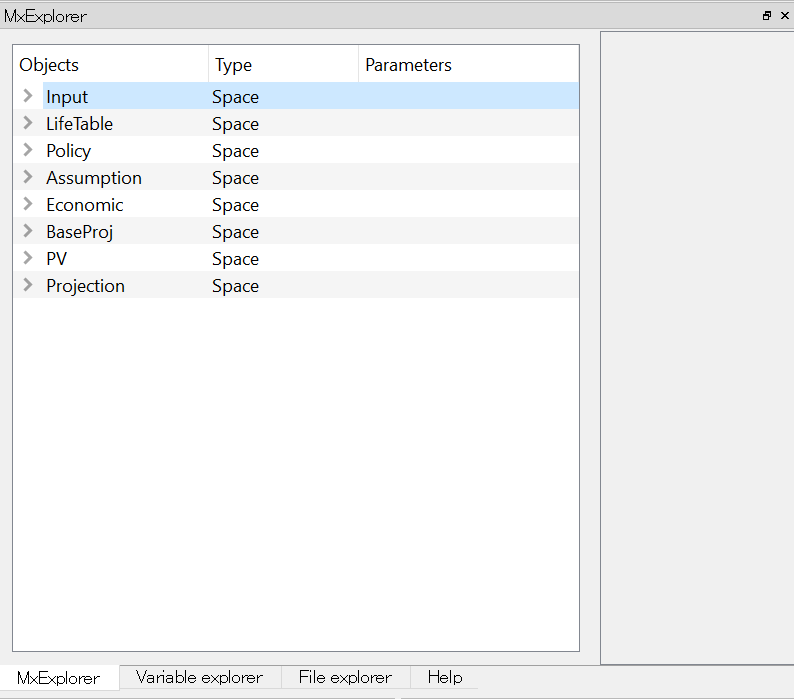
After model is built successfully, The objects that compose model object are shown as a tree in the MxExplorer.

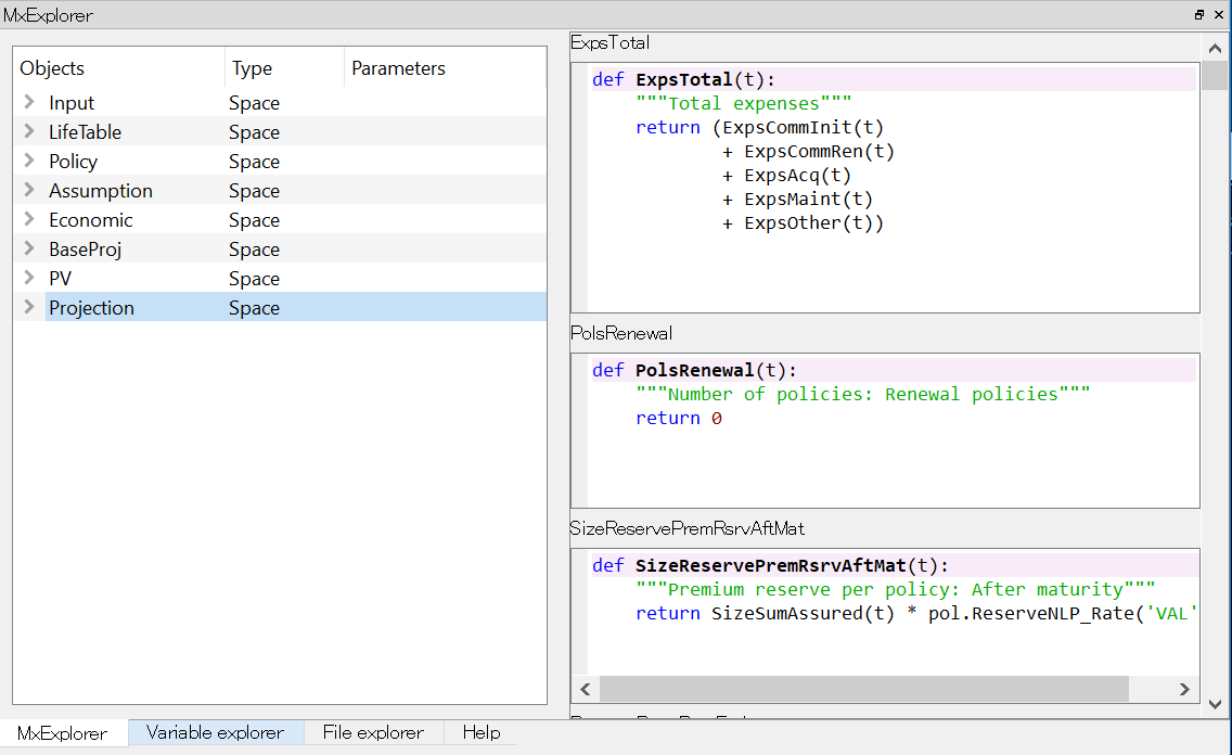
By selecting a space in the MxExplorer and right clicking and selecting Show Formulas in the context menu, the formulas of the cells in the selected space are listed next to the model tree in the MxExplorer.

Run Projection

By default, simplelife model is set up for you to carry out projections and store results by policy under Projection. The attributes of the sample policies are defined on PolicyData tab in Input.xlsm.

To calculate net liability cashflow of the Policy 1 from time 0 to 15:

>> proj = model.Projection[1]
>> result = [proj.NetInsurCF[t] for t in range(16)]

The first line of the above creates Projection[1] space under Projection for the Policy 1, and assign a shorter name to it for convenience. The second line calculate net liability cashflow of the Policy 1 for 15 years (from time=0 to 15) and store the results in a list result. To see the values, type result:

>> result
[-2090.721539115584,
 1593.887335778444,
 1403.8230981682598,
 1247.2761938300212,
 1113.2288348112097,
 1106.8034770880981,
 979.7641693356699,
 857.345650426334,
 745.0110777520256,
 649.2535254400561,
 567.927885159707,
 496.5241286816653,
 431.8978250326952,
 371.9666103072977,
 317.486904907175,
 0.0]

A dynamic space for the Policy 1 appears in the model tree:

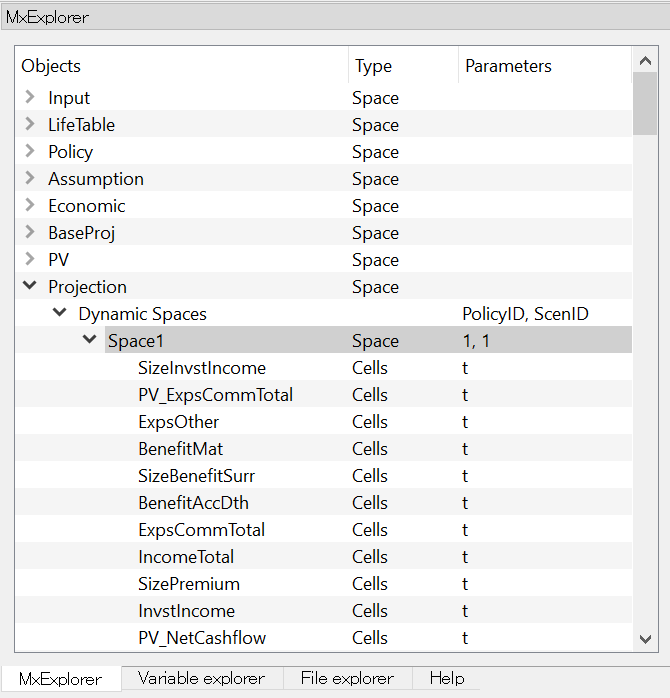
You can see under Dynamic Spaces under Projection space, a space for policy No. 1 (PolicyID=1, ScenID=1) is created.

Output to Pandas objects

By calculating NetInsurCF cells, other cells that the NetInsurCF directly or indirectly refers to are also calculated. To get the values of all cells in a space, access frame property of the space, which returns the values of all the child cells as Pandas DataFrame object:

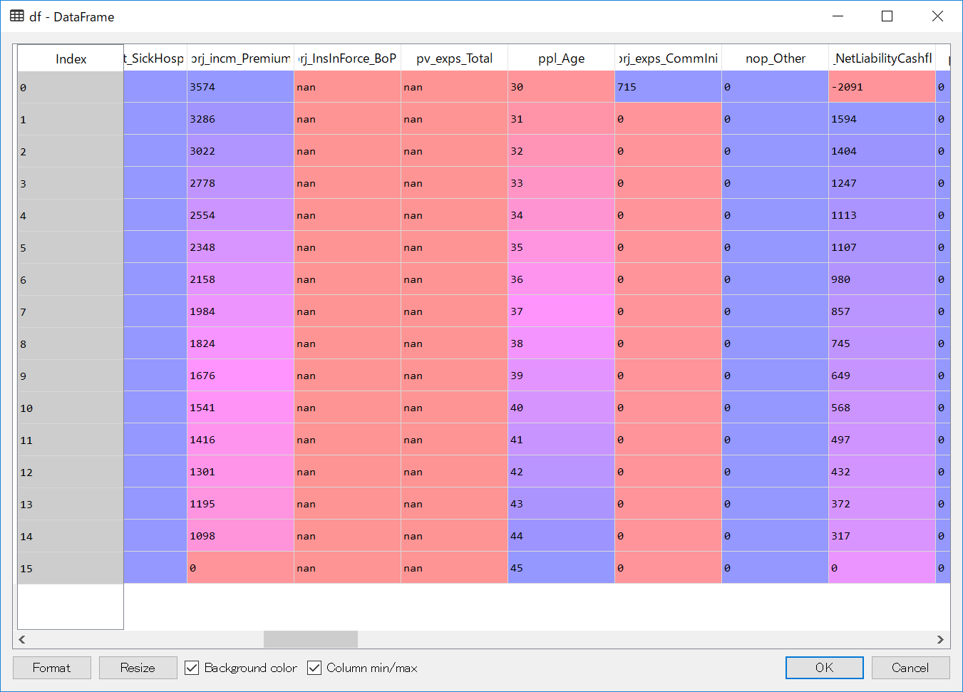
>> df = proj.frame

Pandas is a widely-used data analysis library for Python that provides feature rich data types for data manipulation, such as DataFrame.

To see the contents of df the DataFrame object we have just created, bring up Variable explorer tab on the top right side of the Spyder window, then click on df row.

There are many Pandas tutorials and books out there for you to learn how to slice and dice the data as you like.

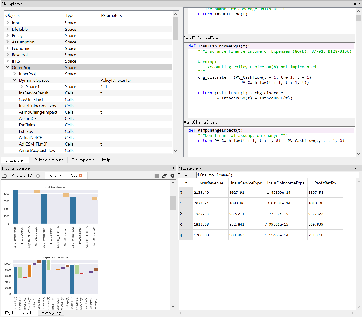
Another way to view data in a tabular form is to use MxDataView from Spyder plugin for modelx.

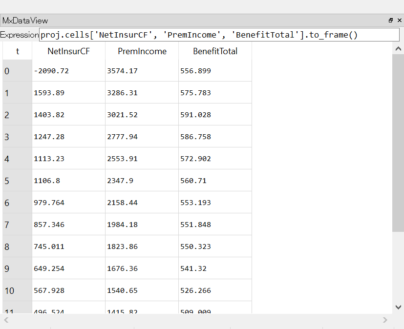
You can see in the figure above that the following Python expression is entered in the text box labeled Expression:

proj.cells['NetInsurCF', 'PremIncome', 'BenefitTotal'].to_frame()

The expression is re-evaluated every time a command in MxConsole is executed, so the data in table is always up to date.

Run Sample Scripts

By default, the project folder also contains sample scripts. Files whose names start with plot_ are the sample scripts that are on Gallery of Examples pages.

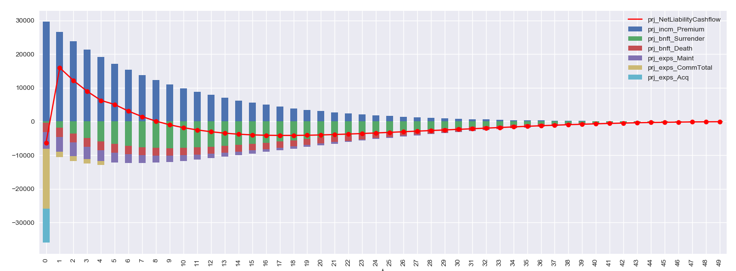
Let’s run a sample script to draw a graph of liability cashflows.

In Spyder, open plot_simplelife.py file in the project folder, from File menu or from File explorer and Run it. The grpah below shows up in another window.

After execution of the script, the session will move to interactive mode. The session is available in an IPython console in Spyder for you to interface with the created model.

The Projection space becomes available as a global variable proj in the MxConsole:

>>> proj
<Space Projection[171, 1] in lifelib>