Quick Start
This is Quick Start guide walk you through steps from setting up a Python environment for lifelib to running a sample model. In this guide, you will see how to:
- Prepare Python environment for lifelib,
- Install lifelib,
- Create your project using a command,
- Build a model by running a script in the project
lifelib models are built in the form of modelx objects. Refer to modelx documentation when you have questions about modelx as you proceed with this tutorial.
To learn Python itself, there are many good tutorials out there on the web, such as the one on Python’s official web site.
This guide assumes users are on Windows platform, but lifelib runs on Linux, and probably on Mac as well although it’s not tested.
Installation
Set up Python Environment
You need to set up a Python environment to use lifelib. Downlowd and install Anaconda distribution. You must install Python 3.x version, not Python 2.7 version. lifelib does not work with Python 2.7. If you already have Anaconda installed, make sure the Python version is 3.4 or newer. Anaconda is a bundle of Python, its major packages and IDEs including packages required or optionally used by for lifelib, such as openpyxl, pandas, Spyder, and provides a Python environment out-of-the-box, just by installing it with few clicks.
Microsoft Excel is not required. You would only need Excel or its alternatives if you want to edit input data files.
Configure Spyder
There are 2 Spyder settings that you want to consider changinig from their default values. Note that you need to restart Spyder to biring your changes into effect.
Disable User Module Reloader
From the Spyder menu, select Tools->Preferences to bring up Preferences window. Choose Python interpreter in the left pane, and you’ll find an area titled User Module Rloader (UMR) on the bottom right side of the Preferences window. Uncheck Enable UMR option to disable User Module Reloader. This prevents Spyder from reloading modelx module every time you re-run the same script from Run menu. Reloading modelx module creates multiple instances of modelx systems within the same Python process, causing models created before and after a reload to reside in different modelx systems.
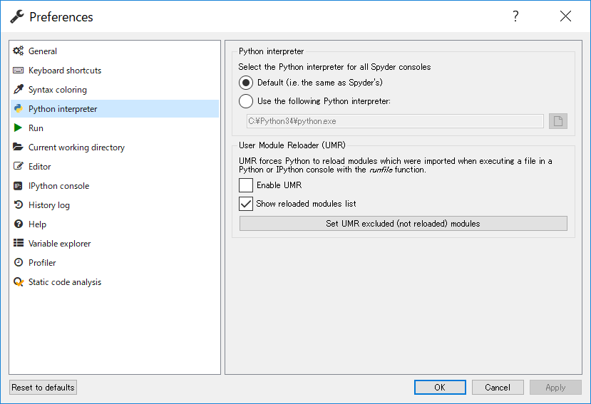
User Module Reloader setting
Graphic Backend
By defult, Graphic Backend option is set to Inline. This option affects where graphs are placed, and how modelx GUI widgets behaves.
If Graphic Backend is set to Inline, graphs are embedded in the IPython console as an output. If it is set to Automatic, graphs are drawn in separate windows, which pop up upon calling plot methods on matplotlib objects.
If Graphic Backend is set to Inline, show_tree function shows
the model tree, blocking the IPython interpreter until you close
the tree window.
If it is set to Automatic, show_tree does not work,
and you need to use get_tree instead:
tree = get_tree(model)
tree.show()
The tree window does not block the interpreter.
To change Graphic Backend option, go to Tools->Preferences, and on the left side of the Preferences window, select IPython console then Graphics tab on the right pane.
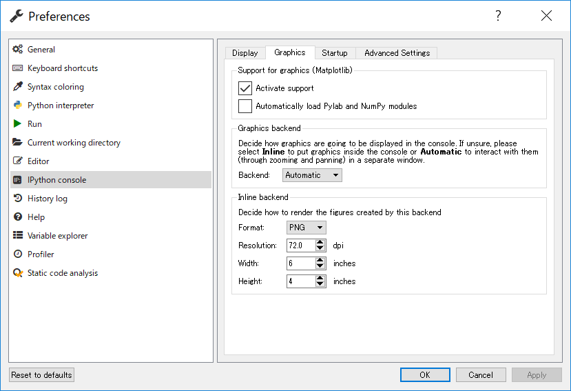
Graphics Backend setting
Install lifelib
lifelib is avalable on PyPI - the Python Package Index.
To install lifelib, use pip command from an Anaconda command prompt.
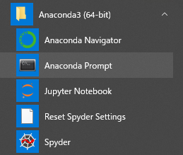
Go to Windows menu and
start Anaconda Prompt inside Anaconda3 submenu to bring up a command prompt.
Then in the Anaconda Prompt, execute the following command:
> pip install lifelib
When you update your existing installation to the newest release, use -U option:
> pip install -U lifelib
The command also installs modelx the package lifelib depends on. All the other required or optionally used packages are included in Anaconda, so no need to install them separately.
Note
(For advanced users) To install the latest development version instead of the released version, clone the lifelib repository and modelx repository on github, and install them from the cloned repos in editable mode.
First Project
Now that you have installed all the programs and packages needed, Let’s start using lifelib.
Create a Project
First, you create your own project folder. A lifelib project is a folder containing source files and data to build a model.
A command lifelib-create helps you create a new project folder
by copying a template project from within the lifelib package to your desired
folder path.
For example, to create a project folder named
mylife under the path C:\Users\fumito by copying lifelib’s default project
template simplelife,
type the following command on the Anaconda prompt:
> lifelib-create --template simplelife C:\Users\fumito\mylife
Alternatively, since simplelife is the default template,
you can get away with –template option like this:
> lifelib-create C:\Users\fumito\mylife
Check that the folder is created and populated with files copied from lifelib’s default project.
Build a Model
Building a model is a process to construct a Model object in a live Python session from script and source files in your project folder.
By default, you have a project module in your project folder, which has
the same name as the project name, such as
simplelife.py.
To build a model, import the project module into a Python session and
call build function in the module. Let’s see how this can be
done in Spyder.
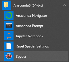
Go to Windows menu, launch Spyder inside Anaconda3 menu.
You’ll find File explorer in the upper right pane of the main Spyder window. Bring it up and navigate to your project folder. By doing so, the working directory(folder) of the IPython console in the bottom right pane is set to the project folder. Then, Type:
>>> import simplelife
>>> model = simplelife.build()
Instead of directly typing the code in the console, you can create a Python script in your project folder, write the code in the script using Editor pane on the left side of the window, and Run it by clicking the green play button in the tool bar. The script is executed in the console on the bottom right side.
During the build, messages appear as the input file is read in. The next time
you build the model, you can pass True as load_saved parameter
of the build function to save loading time:
>>> model = simplelife.build(load_saved=True)
Show Model Tree
Let’s see if the model is built by showing a model tree. By typing in the following code in the console, another window opens.
>>> import modelx as mx
>>> tree = mx.get_tree()
>>> tree.show()
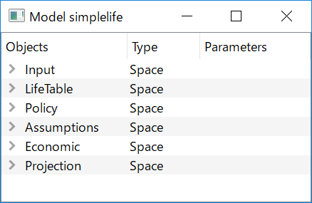
The leftmost Objects column lists child spaces of the model we have just built.
Click on one of the spaces, for example Input,
to open it and see what are inside in the space.
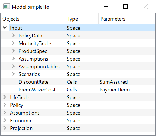
The Objects column now also shows the child spaces and cells of the
Input space.
Run Projection
By default, simplelife model is set up for you to
carry out projections and store results by policy under
Projection. The attributes of the
sample policies are defined on PolicyData tab in Input.xlsm.
To calculate net liability cashflow of the Policy 1 from time 0 to 15:
>> proj = model.Projection[1]
>> result = [proj.NetInsurCF[t] for t in range(16)]
The first line of the above creates Projection[1] space under
Projection for the Policy 1, and assign a shorter name to it for
convenience.
The second line calculate net liability cashflow of the Policy 1 for
15 years (from time=0 to 15) and store the results in a list result.
To see the values, type result:
>> result
[-2090.721539115584,
 1593.887335778444,
 1403.8230981682598,
 1247.2761938300212,
 1113.2288348112097,
 1106.8034770880981,
 979.7641693356699,
 857.345650426334,
 745.0110777520256,
 649.2535254400561,
 567.927885159707,
 496.5241286816653,
 431.8978250326952,
 371.9666103072977,
 317.486904907175,
 0.0]
Let’s see the Projection space for the Policy 1 in the model tree:
>>> tree = mx.get_tree()
>>> tree.show()
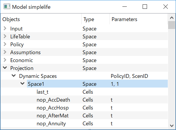
You can see under Dynamic Spaces under Projection space, a space for policy No. 1 (PolicyID=1, ScenID=1) is created.
Output to Pandas objects
By calculating NetInsurCF cells,
other cells that the NetInsurCF directly or indirectly
refers to are also calculated.
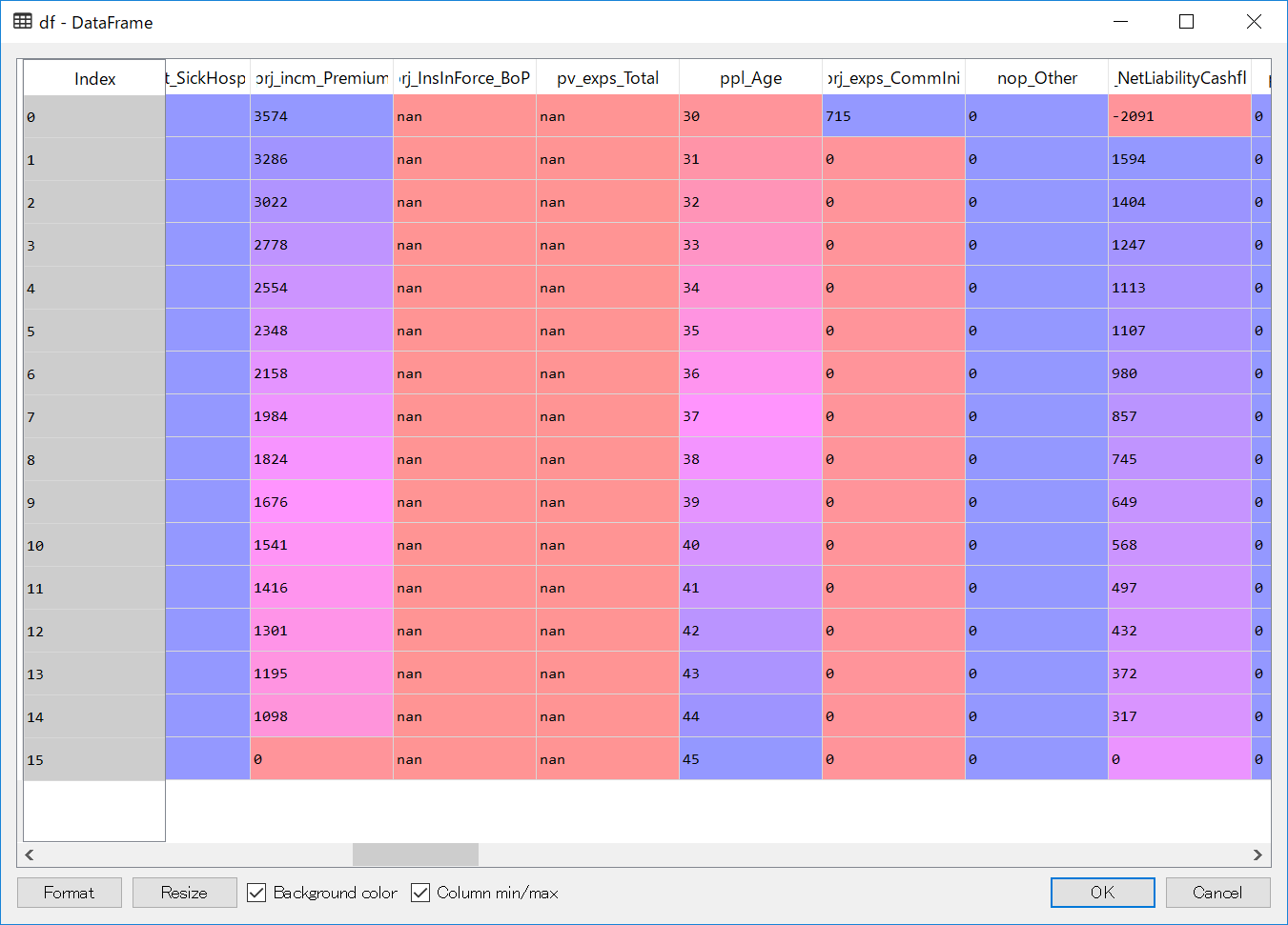
To get the values of all cells in a space, access frame property of the
space, which returns the values of all the child cells as
Pandas DataFrame object:
>> df = proj.frame
Pandas is a widely-used data analysis library for Python that provides feature rich data types for data manipulation, such as DataFrame.
To see the contents of df the DataFrame object we have just created,
bring up Variable explorer tab on the top right side of the Spyder window,
then click on df row.
There are many Pandas tutorials and books out there for you to learn how to slice and dice the data as you like.
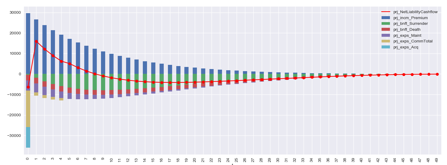
Run Sample Scripts
By default, the project folder also contains sample scripts. Files whose
names start with plot_ are the sample scripts that are on
Gallery of Examples pages.
Let’s run a sample script to draw a graph of liability cashflows.
In Spyder, open plot_simplelife.py file
in the project folder, from File menu or from File explorer
and Run it. The grpah below shows up in another window.
After execution of the script, the session will move to interactive mode. The session is available in an IPython console in Spyder for you to interface with the created model.
The Projection space becomes available as
a global variable proj in the Python console:
>>> proj
<Space Projection[171, 1] in lifelib>