IFRS17 Simulation (Lapse Scenario)
If you’re viewing this page as a static HTML page on https://lifelib.io, the same contents are also available here on binder as Jupyter notebook executable online (it may take a while to load)
To run this notebook and get all the outputs below, Go to the Cell menu above, and then click Run All.
About this notebook
This notebook draws several waterfall charts that show how sources of change in IFRS17 accounts emerge when the actual lapse rate changes at a future point in time and future lapse rate assumptions from that point change accordingly for current-estimate liability valuations at future points.
Those charts are: * Actual cashflows * Present value of expected cashflows * CSM amortization * IFRS17 Financial performance
A notebook for the baseline simulation is also available on lifelib. The baseline simulation assumes that actual cashflow emerge exacltly as esimated at the beginning of simulation.
Warning:
The primary purpose of this model is to showcase the capability of lifelib and its base system modelx, and less attention has been paid to the accuracy of the model or the compliance with the accounting standards. At very least, following items are identified as over-simplification or lack of implementation.
The timing of cashflows is either the beginning or end of each step.
All expenses are included in insurance cashflows.
Loss component logic is not yet incorporated, so
CSMcan be negative.Coverage unit is set to sum assured.
The amortization schedule of acquisition cashflows is constant over time.
All insurance cashflows are considered non-market sensitive, i.e. no TVOG is considered.
Risk adjustment is not yet modeled.
How to use Jupyter Notebook
Jupter notebook enables you to run a Python script piece by piece. You can run each piece of code (called a “cell”) by putting the cursor in the cell and pressing Shift + Enter, and get the output right below the input code of the cell. To learn more about Jupyter Notebook, this tutorial will help you. There are also plenty of other resources on the internet as Jupyter Notebook is quite popular.
You can play around with this notebook, by changeng input values and formulas, re-running code and checking how output tables and charts change accodingly. Note that change in code in one cell may change the results of other cells. To reflect change in one cell on the output of other cells, the other cells need to be re-run after the change.
Initial set-up
The first line %matplotlib notebook, is for specifying drawing mode.
The next few lines are import statements, by which functions defined in other modules become avaialbe in this script.
ifrs17sim and draw_charts modules are in the project directory
of this project. To see what fiels are in the project directory, select
Open from the File menu in the tool bar above.
Building the model
The next line is to create a model from build function defined in
ifrs17sim module which has just been imported.
By supplying True to load_saved parameter of the build
function, the input data is read from ifrs17sim.mx, the ‘pickled’
file to save loading time. To read input from input.xlsm, call
build with load_saved=False or without any parameter because
False is the default value of load_saved.
If you run this code multiple time, the previous model is renamed to
ifrs17sim_BAK*, and a new model is created and returned as
model.
In model thre is a space called OuterProj and other spaces.
OuterProj is parametrized by Policy ID, i.e. each of the spaces with
parameters corresponds to a projection of one policy. For example,
model.OuterProj[1] return the projection of policy ID 1,
model.OuterProj[171] return the projection of policy ID 171.
The first line below sets proj as a shorthand for the projection of
Policy ID 1. You can change the sample policy by supplying some other
ID.
In [2]:
model = ifrs17sim.build(load_saved=True)
proj = model.OuterProj[1]
inner = proj.InnerProj
Adjusting lapse rates
By defalut, base lapse rates are read in from the input file. The initial rates are constant at 8%.
In [3]:
proj.asmp.SurrRate.to_frame(range(6))
Out[3]:
| SurrRate | |
|---|---|
| y | |
| 0 | 0.08 |
| 1 | 0.08 |
| 2 | 0.08 |
| 3 | 0.08 |
| 4 | 0.08 |
| 5 | 0.08 |
In this model, adjustments to the base lapse rates can be made through
the cells SurrRateMult. The cells SurrRateMult in outer and in
inner spaces have have different formulas.
For the outer actual simulation, as seen in the formula below,
SurrRateMult is set to 1 by default, but can be overwritten by user
input. If the user overwrite SurrRateMult(t), then the new value
applies from t goint forward.
In [4]:
proj.SurrRateMult.formula
Out[4]:
def SurrRateMult(t):
    """Surrender rate multiple for the outer projection (Default: 1)"""
    if t == 0:
        return 1
    else:
        return SurrRateMult(t-1)
For the inner projectins, SurrRateMult is set to the same value as
the outer simulation at time 0.
At each step of outer simulation(t0), the lapse rates for the
inner projection starting at t0, are set to the lapse rate of the
actual(outer) simulation applied in the previos period (from t0-1 to
t0)
In [5]:
inner.SurrRateMult.formula
Out[5]:
def SurrRateMult(t):
    """Surrender rate multiple for the inner projection (Default: 1)"""
    if t == 0:
        return outer.SurrRateMult(t)

    elif t == t0:
        return _space.parent(t-1).SurrRateMult(t-1)

    else:
        return SurrRateMult(t-1)
We assumes that the actual lapse rate doubles from time 2, i.e. the beginning of the 3rd year, and continues to be doubled. Accordingly, we assume we double our lapse rate assumption from the end of the 3rd yer, one year later later than the change in actual lapse.
In [6]:
proj.SurrRateMult[1] = 1
proj.SurrRateMult[2] = 2       # Actual lapse rate from t=2

inner[1].SurrRateMult[1] = 1
inner[2].SurrRateMult[2] = 1
inner[3].SurrRateMult[3] = 2   # The lapse assumption for estimated cashflows at t=3 and thereafter
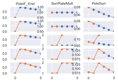
The figure below shows how underlying poicies change over time. The 3 columns in the fiture represents 3 cells, and filled lines denote actual(outer) while the dotted lines denote expected(inner). For each column, rows from the top to the bottom represent the time steps of the outer simulation, stating at time 0.
The leftmost column is the graph of policies in-force at the end of each
period. The column in the middle shows how SurrRateMult for actual
lapse rate and estimated lapse rates change over time. SurrRateMult
stays at time 0 and 1 (1st and 2nd rows). Then it doubles for the acutal
at time 2 (3rd row), while the estimate stays still at 1 for 1 year.
Then the estimate catches up the actual at time 3 (4th row).
The right most column show the movement in terms of the number of surrender policies.
In [7]:
draw_actest_pairs(proj, inner, ['PolsIF_End', 'SurrRateMult', 'PolsSurr'], 5, 5)
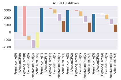
Actual cashflows
The code below generates a waterfall chart that simulates actual insurance cashflows that are assumed to be equal to the expected. The net asset balance is reset to zero at the end of each period, so the assets are equal to the liabilities at the beginning of each period. The assets are held as cash, and bear interest at the same rate as discount rate.
In [8]:
proj.IntAccumCF.formula
Out[8]:
def IntAccumCF(t):
    """Intrest on accumulated cashflows"""
    return (AccumCF(t)
            + PremIncome(t)
            - ExpsTotal(t)) * DiscRate(t, 0)
In [9]:
actcf = get_waterfalldata(
            proj,
            items=['PremIncome',
                   'IntAccumCF',
                   'ExpsAcqTotal',
                   'BenefitTotal',
                   'ExpsMaintTotal',
                   'ActualNetCF'],
            length=4,
            reverseitems=['ExpsAcqTotal',
                          'BenefitTotal',
                          'ExpsMaintTotal'])

actcf
Out[9]:
| PremIncome | IntAccumCF | ExpsAcqTotal | BenefitTotal | ExpsMaintTotal | ActualNetCF | |
|---|---|---|---|---|---|---|
| t | ||||||
| 0 | 3574.169909 | -23.007341 | -4072.250973 | -556.898777 | -1035.741699 | -2113.728881 |
| 1 | 3286.309839 | -15.774573 | -164.315492 | -575.782913 | -952.324098 | 1578.112762 |
| 2 | 3021.518710 | -10.000811 | -151.075936 | -661.304449 | -875.591536 | 1323.545979 |
| 3 | 2536.214461 | -4.600831 | -126.810723 | -614.423546 | -734.957526 | 1055.421834 |
In [10]:
draw_waterfall(actcf, stocks=[0, 5], title='Actual Cashflows')
Out[10]:
<matplotlib.axes._subplots.AxesSubplot at 0x27dd0f21e80>
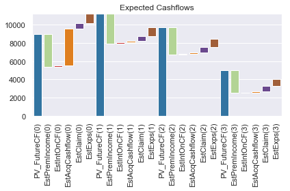
Present value of expected cashflows
The code below generate a waterfall chart that shows how the present value of expected insurance cashflows unwinds over time.
The waterfall bars are disconected at t = 3, because we change the lapse assumption there. The present value of future cashflows decrease due to the decrease in future policies.
In [11]:
estcf = get_waterfalldata(
            proj,
            items=['PV_FutureCF',
                   'EstPremIncome',
                   'EstIntOnCF',
                   'EstAcqCashflow',
                   'EstClaim',
                   'EstExps'],
            length=4,
            reverseitems=['EstPremIncome'])

estcf
Out[11]:
| PV_FutureCF | EstPremIncome | EstIntOnCF | EstAcqCashflow | EstClaim | EstExps | |
|---|---|---|---|---|---|---|
| t | ||||||
| 0 | 8954.018303 | -3574.169909 | 157.317616 | 4072.250973 | 556.898777 | 1035.741699 |
| 1 | 11202.057458 | -3286.309839 | 135.485808 | 164.315492 | 575.782913 | 952.324098 |
| 2 | 9743.655931 | -3021.518710 | 116.232070 | 151.075936 | 591.028140 | 875.591536 |
| 3 | 5040.473472 | -2536.214461 | 50.490409 | 126.810723 | 614.423546 | 734.957526 |
In [12]:
draw_waterfall(estcf, title='Expected Cashflows')
Out[12]:
<matplotlib.axes._subplots.AxesSubplot at 0x27dd2c92748>
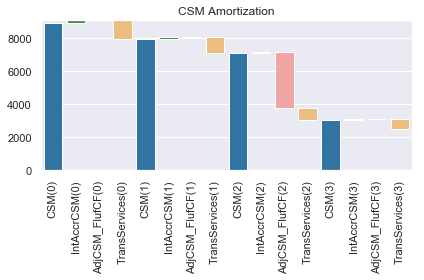
CSM amortization
The CSM amortization chart below depicts items that increase/decrease CSM balance.
The adjustment to CSM for changes in fulfilment cashflows
(AdjCSM_FlufCF) is negative in the 3rd period. This offsets to a
great extent the decrease in PV_FutureCF in the chart above (or
increase in liability, if PV_FutureCF is negative unlike this
sample, which is often the case)
AdjCSM_FlufCF takes the difference of PV_Cashflows with
different parameters.
PV_Cashflow(t+1, t+1, 0) starts projection at t+1 into the
future using the lapse assumption updated at t+1, and discount the
cashflows using the discount rate fixed at time zero, back to time
t+1.
PV_Cashflow(t, t+1, 0) starts projection at t into the future
using the lapse rate assumption before the change, and discount the
cashflows using the discount rate fixed at time zero, back to time
t+1.
The sources of difference between these valuese are the difference in
the number of policies in-force, and the difference in future laps
rates, which impact projected policies in-force and cashflows from
t+1.
In [13]:
proj.AdjCSM_FlufCF.formula
Out[13]:
def AdjCSM_FlufCF(t):
    """Adjustment to CSM for changes in fulfilment cashflows (44(c)->B96-B100)

    Warnings:
        Only B96(b) changes in PV of the future cashflows are implemented.

    TODO: Risk Adjustment is yet to be implemented. At the momement
    this adjustment only considers present value of future cashflows.

    TODO: Loss component for onerous contracts are yet to be implemented.
    At the momemnt this adjustment allows negative CSM.
    """

    return PV_Cashflow(t + 1, t + 1, 0) - PV_Cashflow(t, t + 1, 0)
In [14]:
csmrf = get_waterfalldata(
            proj,
            items=['CSM',
                   'IntAccrCSM',
                   'AdjCSM_FlufCF',
                   'TransServices'],
            length=4,
            reverseitems=['TransServices'])

csmrf
Out[14]:
| CSM | IntAccrCSM | AdjCSM_FlufCF | TransServices | |
|---|---|---|---|---|
| t | ||||
| 0 | 8954.018303 | 134.310275 | 0.000000 | -1107.579599 |
| 1 | 7980.748979 | 119.711235 | 0.000000 | -1018.376245 |
| 2 | 7082.083968 | 106.231260 | -3415.591431 | -713.418589 |
| 3 | 3059.305208 | 45.889578 | 0.000000 | -598.832149 |
In [15]:
draw_waterfall(csmrf, title='CSM Amortization')
Out[15]:
<matplotlib.axes._subplots.AxesSubplot at 0x27dd2e54320>
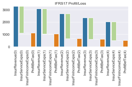
IFRS17 Financial performance
The chart below simulates P&L accounts based on IFRS17 from the
background data used to draw the charts above. The profit in each period
is released and the outstanding net balance (NetBalance) is reset to
zero.
The profit in the 3rd period is decreased due to the adverse change in lapse assumption, but its impact on the current profit is limited because of the offset between the change in CSM and the PV of future cashflows.
In [16]:
proj.InsurRevenue.formula
Out[16]:
def InsurRevenue(t):
    """Insurance Revenue (82-85, B120-B125)"""
    return (EstClaim(t)
            + EstExps(t)
            + RelsRiskAdj(t)
            + TransServices(t)
            + AmortAcqCashflow(t)
            - AdjLCO_FulfCF(t))
In [17]:
proj.InsurServiceExps.formula
Out[17]:
def InsurServiceExps(t):
    """Insurance Service Expense (103(b))"""
    return (IncurClaim(t)
            + IncurExps(t)
            + AmortAcqCashflow(t)
            + Incr_LossComp(t)
            - AdjLCO_FulfCF(t))
In [18]:
ifrspl = get_waterfalldata(
            proj,
            items=['InsurRevenue',
                   'InsurServiceExps',
                   'InsurFinIncomeExps',
                   'ProfitBefTax'],
            length=5,
            reverseitems=['InsurServiceExps'])
ifrspl
Out[18]:
| InsurRevenue | InsurServiceExps | InsurFinIncomeExps | ProfitBefTax | |
|---|---|---|---|---|
| t | ||||
| 0 | 3264.948734 | -2157.369136 | 1.421085e-14 | 1107.579599 |
| 1 | 3065.729235 | -2047.352990 | -3.019807e-14 | 1018.376245 |
| 2 | 2657.446518 | -2014.304238 | 1.776357e-15 | 643.142280 |
| 3 | 2348.942071 | -1750.109922 | 2.664535e-15 | 598.832149 |
| 4 | 2014.874787 | -1512.241430 | 2.886580e-15 | 502.633357 |
In [19]:
draw_waterfall(ifrspl, stocks=[0, 3], title='IFRS17 Profit/Loss')
Out[19]:
<matplotlib.axes._subplots.AxesSubplot at 0x27dd30f6da0>